2.1 A Conventional Approach: Propensity Scores and Balance
In a randomised control trial (RCT), researchers believe treatment and control groups are similar because of randomisation. In this case, the similar groups are compatible and should not have systematic differences. In observational data, the exposure to a treatment is unlikely to be random, implying there may be systematic differences between groups. Systematic differences refer to consistent variations or disparities between groups in the study. These differences are not due to random chance but rather indicate a pattern or trend, perhaps due to selection-bias. As groups are not comparable, Equation 1.3 leads to a biased estimate of the treatment effect.
For example, consider the causal question: “How much does obtaining a bachelors degree increase lifetime earnings?”. Individuals who complete a bachelor’s degree are not selected at random for university programs (treatment) and may have different observable attributes than those who do not attend a university (control). Perhaps those who attend university have higher academic abilities, higher motivation, or grew up with parents with higher income. Because of these systematic group covariate differences, a simple comparison of mean income could lead to attributing university attendance as the cause of higher incomes when the effect is confounded by the differences in covariates between groups. In this example, the confounding covariates are academic ability, motivation, and parental income that impact the probability of someone obtaining a bachelors degree. This discussion introduces the idea of covariate balance which is a key concept behind underlying propensity score methods.
Note 2.1: What is Covariate Balance
Covariate balance is the idea that covariates are approximately equivalent across treatment and control groups. If the distribution of each covariate is the same across each group, then the covariates are balanced and a meaningful comparison between groups can be made. Equally, similar covariates across groups implies exchangability as the two groups should be similar (thus can be exchanged). There is a conceptual link between covariate balance, unconfoundedness, and exchangeability meaning that Equation 1.6 is satisfied when covariates are balanced.
In the bachelor’s degree example, suppose that comparable treatment and control individuals are matched together to create balanced pairs. Between these pairs, covariates are balanced such as the same academic ability, motivation, parental income, geographic residence etc. The covariates are said to be conditioned on by matching individuals on these covariates. Comparing the balanced matched pairs should result in a robust estimate of a bachelors degree’s impact on earnings because the individuals are exchangeable and satisfy Equation 1.7. However, practically this matching is difficult to perform as exact matches cannot be made as the number of covariates increases. For example, finding two people with the same gender is simple but finding two people with the same gender, age, education, income, motivation, location, experience, and race is nearly impossible. Thus, there is a dimensionality problem as the dimension of the number of covariates increases.
Rosenbaum and Rubin (1983) offer a valuable tool for analysing observational data called the propensity score. The propensity score is the probability of treatment assignment conditioned on observed covariates. Essentially, the propensity score reduces the dimension of the number of covariates to a single dimension to avoid the dimensionality problem. Let the propensity score be denoted as \(e(X)\) and be expressed as:
\[
e(X)=P(T=1|X=x).
\tag{2.1}\]
A prediction of the conditional probability of treatment on covariates is a good summary of the covariate’s effect on receiving the treatment. The covariate imbalance between bachelors degrees and controls arose from people self-selecting themselves into a bachelors degree programme because of these covariates. For example, people with higher motivation and academic ability are more likely to go to university. If it is the covariates that impact the probability of going to university, then a prediction of the probability of going to university based on these covariates should summarise the covariate effects.
It is hoped that conditioning on this propensity score should balance the data and meet the conditional independence assumption stated in Equation 1.7. There are many sources that offer a comprehensive guide to propensity score methods such as (Cunningham 2021, chap. 4) who provides applications and coded examples in R, Python, and Stata.
Note 2.2: Balance and Propensity Scores
Note that an RCT will satisfy Equation 1.6 as randomisation implies the potential outcomes are independent of the treatment assignment. Propensity score methods aim to satisfy Equation 1.7 as the potential outcomes are independent of the treatment status conditioned on some covariates. Thus, \(Y(1), Y(0) \perp \!\!\! \perp T\mid X\) is satisfied by \(Y(1), Y(0) \perp \!\!\! \perp T\mid \widehat{e(X)}\).
Conditioning on the propensity score aims to replicate an RCT in observational data by balancing covariates between groups. When observations are conditioned on their propensity score, differences in outcomes can be confidently attributed to the treatment itself, rather than to pre-existing differences in covariates.
Two common methods that use propensity scores are propensity score matching (PSM) and inverse propensity weighting (IPW).1 PSM creates matched sets with similar propensity scores. IPW creates a balanced pseudo-population, where observations are weighted on the inverse of the propensity score. The pseudo-population is created by up-weighting observations with a low propensity score and down-weighting observations with a high propensity score.
At a high level, the conditioned property of the propensity score is translated into a model by using PSM or IPW. King and Nielsen (2019) provide a notable criticism of propensity score matching, which is a very interesting read. In the following examples, IPW is used due to theoretical advantages and ease of software implementation.
2.1.1 Assessing balance
Balance assessment is an important step to ensure that conditioning on the propensity score has been successful. A commonly recommended measure of covariate balance is the standardised mean difference or SMD. This is the difference in the mean of each covariate between treatment groups standardised by a standardization factor so that it is on the same scale for all covariates.
SMDs close to zero indicate good balance. P. Austin (2011) notes that \(0.1\) is a common threshold for determining if a variable is balanced. This threshold is a guideline to the approximate region that indicates a covariate is balanced and should not be interpreted as a binary rule. Additionally, a variance ratio below 2 is generally acceptable. For brevity, my analysis only considers the SMD.
2.1.2 Propensity Score Modelling with Logistic Regression
A conventional propensity score model uses logistic regression to predict a probability between \(0\) and \(1\). Models may be specified to include interaction terms and polynomial terms to capture complex trends in the data. There are a range of approaches for specifying a propensity score model, but the process is a heuristically driven art rather than science. (see Brookhart et al. 2006; Heinrich, Maffioli, and Vázquez 2010). One suggestion is to include two-way interaction terms between covariates and squared terms and then remove terms which are not statistically significant. Notably, many researchers do not discuss the specification of propensity models in their papers. P. C. Austin (2008) reviews \(47\) papers that use propensity scores and find few perform adequate model selection, assess balance, or apply correct statistical tests.
It is important to note that the true propensity score is never observable. A propensity score that is close to the theoretically true probability is well calibrated. Poorly calibrated propensity scores may result in poor balance and biased estimation of the treatment effect. Propensity scores may be poorly calibrated as covariates may be omitted by error, poorly measured, or be unobservable. Logistic regression may not predict calibrated scores if the true relationship is non-linear or involves complex interactions between covariates. Another important note is that the propensity model itself does not have an informative causal interpretation. In logistic regression, the coefficients are the log-odds of the treatment assignment for each variable which is not informative of the desired estimand.
The first application of machine learning in causal inference was to predict propensity scores. Despite this, logistic regression still appears to be the most common model for predicting propensity scores.
2.2 Probability Machines: Probability Theory and Machine Learning
Supervised machine learning usually focuses on classifying observations into groups, or predicting continuous outcomes. Probability prediction is a hybrid of these tasks, aiming to predict the continuous probability an observation belongs to a certain class. Machine learning methods that predict probabilities are sometimes called probability machines.
Probability machines are valuable in applications requiring calibrated probability predictions. For example, probability machines can predict loan defaults or other adverse events in finance. In marketing, they estimate the likelihood of customer response to a campaign. Gamblers and bettors want robust probability predictions to enhance their betting strategies. Probability machines can be applied wherever calibrated probability predictions are needed.
Probability machines offer many advantages over parametric methods like logistic regression:
Improved Calibration: Probability machines often provide better-calibrated predictions by capturing complex data relationships.
Flexible Modelling: Unlike parametric methods like logistic regression, probability machines don’t rely on assumptions of additivity or linearity, allowing them to model intricate relationships that parametric models miss.
Efficient Feature Selection: These machines automatically select features, making them ideal for high-dimensional datasets where manual selection is impractical.
Handling Missing Data: Probability machines handle missing data robustly, minimizing the need for extensive data reprocessing and imputation.
Simplified Data Exploration: By exploring complex data structures in a data-driven way, probability machines simplify model specification. For instance, tree-based models remain unaffected by adding squared or interaction terms, streamlining the modeling process.
In causal inference, probability machines can predict better calibrated propensity scores and better estimate treatment effects. This discussion aims to clarify the use of probability machines in causal inference given the unique requirements of propensity score specification. Probability machines are theoretically complex and there are unanswered questions in this space.
Note 2.3: A Particularly Important Method: Classification and Regression Trees
Moving forward, a particularly important model is the Classification and Regression Trees. Breiman et al. (1984) introduces method, commonly known as CART, that partitions data according to a splitting criterion, resulting in an “if this, then that” interpretation. CART models are also widely known as a decision trees. The splits are recursive, meaning splits are applied upon previous splits, such as trees breaking into branches and then leaves. The splits are also greedy as each potential split only considers information available at that split instead of past or future splits. Each parent node is split to create two child nodes and the final nodes of a CART model are called terminal nodes.
For example, when classifying pets into cats versus dogs, the first split might be“if barks” and the second is “heavier than 5 kg”. The tree says If it barks and is heavier than 5 kg, then it is a dog.
A single classification tree typically uses the Gini index to determine its splits. Each split aims to maximise node purity, meaning the nodes contain the highest possible proportion of one class. The Gini index measures impurity, with lower Gini values indicating higher purity. Intuitively, the aim of a classification tree’s loss function is to minimise the misclassification rate of observations. By selecting splits that reduce the Gini index, the tree minimises classification error and increases accuracy.
2.2.1 Choice of Loss Function and Probability Prediction
The loss function measures the difference between a model’s predictions and the actual target values, serving as a measure of a model’s performance. Different loss functions influence a model’s behaviour so the choice of loss function is important. Classification models predict the category that each observation belongs to not the probability of each class. For instance, in fraud detection, banks use classifiers to distinguish between fraudulent and routine transactions. Many classification loss functions minimise classification errors and improve accuracy as this results in the best classification. A loss function like the Gini index is effective for classification problems but it is unclear if this applies to probability problems. In other words, minimizing misclassification error may not lead to accurate probability predictions.
At a high level, to classify an observation, \(x_i\) as an \(A\) or \(B\), a model needs to determine if \(\Pr(x_i=A)\) is less than or greater than \(0.5\). If \(\widehat{\Pr}(x_i=A) > 0.5\), then it is more likely to be an \(A\) and if \(\widehat{\Pr}(x_i=A) <0.5\) then it is more likely to be a \(B\). Thus, if \(x_i\) is an \(A\), it is trivial if \(\widehat{\Pr}(x_i=A)\) is \(0.51\) or \(0.99\) as this makes no difference to the classification as an \(A\). But the difference between \(\widehat{\Pr}(x_i=A) = 0.51\) and \(0.99\) is extreme for a probability machine. It is important to understand that classification models are optimised for classification accuracy rather than probability prediction. This distinction affects the performance of ensemble methods like random forests or bagging ensembles that use classification trees for probability prediction.
2.2.2 Bagging and Random Forest as Probability Machines
Note 2.4: A Quick Note on Ensemble Learning
Ensemble learning refers to a general framework of machine learning that combines multiple simple models to create a better overall model. The philosophy behind ensemble learning is rooted in the wisdom of crowds principle, where the collective decisions from multiple models often outperform that of individual models. Often, ensemble learning methods use multiple CART models.
Bagging ensembles, random forests, and gradient boosting machines are all machine learning methods that combine CART models and are all examples of ensemble learning algorithms. These methods are introduced in the following discussion.
Consider an ensemble method called the lazy ensemble that combines multiple CART trees. Each tree is fitted on the same data without any cross validation. In this ensemble, class probabilities are determined through a vote count method. Within the lazy ensemble, each tree makes a class prediction based on the majority class in a terminal node. For instance, if \(x_i\) lies in a terminal node where \(80\%\) of the observations are classified as an \(A\), that individual tree will classify \(x_i\) as \(A\). The ensemble’s overall prediction for \(x_i\) is derived from the proportion of trees that classify \(x_i\) as \(A\) or \(B\). Thus, the ensemble counts votes for each class across the ensemble. Let \(T\) be the total number of trees and \(b_t\) be the \(t\)-th tree in the ensemble. Let \(\mathbb{I}(b_t(x_i) = A)\) be the indicator function that returns \(1\) when \(b_t\) predicts that observation \(x_i\) belongs to class \(A\). The probability of class \(A\) for observation \(x_i\) is calculated as:
Olson and Wyner (2018) note bias towards predictions of \(0\) or \(1\) when trees in an ensemble framework are highly correlated and a vote count method is used. In the lazy ensemble, each tree is identical and perfectly correlated implying that each tree will make the the same class prediction for each \(x_i\). For such an ensemble, the predicted probabilities will will be exactly \(0\) or \(1\) using a vote count. Of course a lazy ensemble of identical trees would never be used but the intuition still applies in the real world where ensembles may have some degree of correlation. The larger the correlation, the more the probability predictions will exhibit a divergence bias towards \(0\) and \(1\). Notably, divergence bias is not problematic in classification applications, as a larger number of trees correctly classifying the observation is encouraging.
To reduce tree correlation and improve upon the lazy ensemble, a bagging ensemble (see Breiman 1996) trains each tree on a randomly selected bootstrapped sample of the data. Random forests (see Breiman 2001) further reduce tree correlation by considering a random number of variables at each split, commonly referred to as \(mtry\) in software implementations. When \(mtry\) is equal to to number of predictors, the model considers all variables at each split and the random forest is equal to a bagging ensemble. Note that these ensemble methods typically use a vote count method in the same way as the lazy ensemble. A lower \(mtry\) should reduce the correlation between trees and decrease divergence bias as the structure of the tree is modified by the selected variables at each split. However, a lower \(mtry\) also introduces other theoretical problems.
Consider the scenario where the binary outcome (treatment and control) of the ensemble is strongly related to a single predictor and weakly related to other noisy predictors. If \(mtry\) is low then each split may not consider the strong predictor and more commonly splits on weak or noisy predictors. Each predictor has a chance of \(\frac{mtry}{\text{number of predictors}}\) of selection at each split implying a lower \(mtry\) decreases the chance of a splitting on the strong predictor. Splits on the weak or noisy predictors may not result in a meaningful increase in node purity and successive splits may result in impure terminal nodes that poorly predict the class of \(x_i\) in each tree. Such an ensemble may have highly unstable probability predictions.
Additionally, consider there is a class imbalance and the majority of observations are classified as \(A\) not \(B.\) The terminal nodes of each tree within an ensemble are more likely to contain the majority class. Consequently, there is a majority class bias as each tree in the ensemble is more likely to misclassifying an observation as an \(A\) because the terminal nodes have a higher proportion of \(A\) due to the higher proportion of \(A\)’s in the data overall.
Note 2.5: Class Imbalance and Machine Learning
When there is a difference in the number of observations in each class, this is called class imbalance. It is important to note that majority class bias exists in conventional machine learning classification tasks. Bagging ensembles and random forest are well known to be sensitive to class imbalance meaning that class predictions are biased towards the majority (see Bader-El-Den, Teitei, and Perry 2019).
However, the class imbalance problem is particularly notable when predicting probabilities. The probability prediction from a vote count method is very sensitive to a change in the votes from each tree. Suppose that balanced data results in \(80/100\) trees classifying \(B\) as \(B\) and imbalanced data (more \(A\) than \(B\)) reduces correct classifications of \(B\) to \(60/100\). This results in a \(20\%\) margin of error in probability estimates but the classification remains as \(B\).
Individually, a low \(mtry\) can lead to unstable probability predictions and class imbalance can create bias towards the majority class. But probability machines are particularly effected when there is both a low \(mtry\)and class imbalance. Because successive noisy splits (relating to a low \(mtry\)) result in impure child nodes, the effects of majority class bias are exaggerated. Without the ability to separate the classes, the majority class will dominate terminal nodes. If the ensemble was able to split on informative covariates each time (\(mtry\) is higher), then it should still be able to create pure splits even when there is some class imbalance. In other words, if there is a small class imbalance, reducing \(mtry\) may reveal majority class bias not visible at higher \(mtry\)’s. Equally, if there is low \(mtry\), then even a small class imbalance can lead to majority class bias.
As a general philosophy, ensemble learning methods based on classification trees are poor at predicting probabilities. If \(x_i\) has a known membership of \(A\), and an unknown \(\Pr_{\text{true}}(x_i=A) = 0.6\), the ensemble might classify \(x_i\) correctly \(90\%\) of the time leading to \(\widehat{\Pr}(x_i=A) = 0.9\). As a probability machine, the ensemble has overestimated the probability by \(30\%\) even though a \(90\%\) classification accuracy is excellent. To predict \(\Pr_{\text{true}}(x_i=A) = 0.6\), an ensemble needs to incorrectly classify \(x_i\) in \(40\%\) of its trees. However, bagging ensembles and random forests are designed to maximise classification accuracy and there is no incentive for the model to intentionally achieve a specific misclassification rate that aligns with the true probability.
To exemplify these theoretical points, the National Supported Work (NSW) programme is a commonly discussed dataset in causal inference. The data results from a randomised controlled trial with \(445\) total participants, \(185\) in the program group, and \(260\) in the control group, so the true probability of treatment for each individual can be calculated as \(185/445=0.42\) or \(42\%\). Further information about this data is found in Appendix A. Randomisation should ensure that the probability of treatment is independent of the predictors and so all predictors should be noisy or weak. Although Figure 2.2 and Table 3.1 suggest some covariates do have a greater impact on the probability of participating in the programme, which echoes research by Smith and Todd (2005) who suggest randomisation is imperfect in the NSW dataset. Thus, the “best” calibrated probability model will have a distribution centred near \(0.42\) with some noise due to imperfect randomisation.
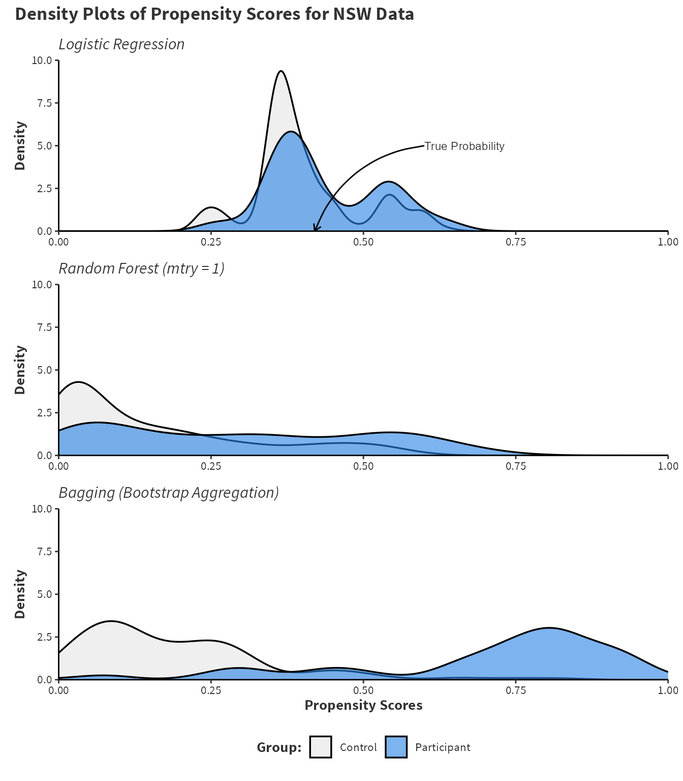
Figure 2.1 shows both divergence bias and majority class bias using randomForest() to fit both the random forest and bagging ensemble. Recall that a bagging ensemble is a random forest model when \(mtry\) is equal to the number of predictors and so specifying mtry = 7 in the randomForest() function fits a bagging ensemble. Additionally, logistic regression using the glm() function provides a meaningful comparison.
# Create Figure 2.1library(randomForest)library(patchwork)library(ggplot2)library(ragg)set.seed(88)nsw_formula <-as.formula(as.factor(treat) ~ age + educ + re75 + black + hisp + degree + marr)logit_preds <-glm(nsw_formula, data = nsw_data, family =binomial())$fitted.values rf_mtry1_preds <-predict(randomForest(nsw_formula, mtry =1, data = nsw_data), newdata = nsw_data, type ="prob")[, 2]bagging_model <-randomForest(nsw_formula, mtry =7, importance =TRUE, data = nsw_data)bagged_preds <-predict(bagging_model, newdata = nsw_data, type ="prob")[, 2]plot_pmachines <-function(pscores, plot_subtitle) {ggplot(nsw_data, aes(x = pscores, fill =factor(treat))) +geom_density(alpha =0.6, linewidth =0.6) +scale_fill_manual(values =c("#e5e5e5", "#2780e3"), labels =c("Control", "Participant")) +labs(subtitle = plot_subtitle, x ="Propensity Scores", y ="Density", fill ="Group:") +scale_x_continuous(expand =expansion(0), limits =c(0,1)) +scale_y_continuous(expand =expansion(0), limits =c(0,10)) + custom_ggplot_theme}p1 <-plot_pmachines(logit_preds, "Logistic Regression") +xlab(NULL) +theme(legend.position ="none") +annotate(geom ="curve", x =0.6, y =5, xend =0.42, yend =0, curvature = .3, arrow =arrow(length =unit(2, "mm"))) +annotate(geom ="text", x =0.6, y =5, label ="True Probability", hjust ="left", color ="#333333", size =3)p2 <-plot_pmachines(rf_mtry1_preds, "Random Forest (mtry = 1)") +xlab(NULL) +theme(legend.position ="none")p3 <-plot_pmachines(bagged_preds, "Bagging (Bootstrap Aggregation)")p1 / p2 / p3 +plot_annotation(title ="Density Plots of Propensity Scores for NSW Data", theme = custom_ggplot_theme)
Figure 2.1: Compares the density estimates of the propensity scores for control and participant groups in the National Supported Work programme. randomForest() fits a random forest with mtry = 1 and bagging ensemble with mtry = 7. The default values of ntree = 500 and nodesize = 1 are used. A logistic regression model is included for a comparison.
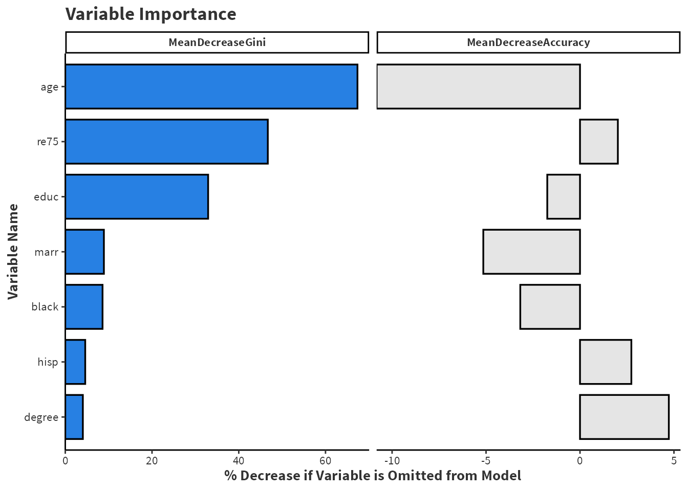
# Create Figure 2.2library(ggplot2)library(tidyverse)imp <-as.data.frame(importance(bagging_model))imp <-cbind(vars =rownames(imp), imp)imp <- imp[order(imp$MeanDecreaseGini),]imp$vars <-factor(imp$vars, levels =unique(imp$vars))imp %>%pivot_longer(cols =matches("Mean")) %>%ggplot(aes(y = vars, x = value, fill = name)) +geom_bar(stat ="identity", width =0.8, show.legend =TRUE, position =position_dodge(width =0.8), color ="black", linewidth =0.6) +facet_grid(~factor(name, levels =c("MeanDecreaseGini", "MeanDecreaseAccuracy")), scales ="free_x") +scale_fill_manual(values =c("#e5e5e5", "#2780e3")) +scale_x_continuous(expand =expansion(c(0, 0.04))) +labs(title ="Variable Importance",x ="% Decrease if Variable is Omitted from Model", y ="Variable Name" ) + custom_ggplot_theme +theme(legend.position ="none")
Figure 2.2: Compares the variable importance assigned to each variable from a bagging ensemble fitted on data from the National Supported Work programme. randomForest() fits a baggin ensemble with mtry = 7 with default ntree = 500 and nodesize = 1.
Figure 2.1 shows the logistic regression model has identified a central tendency and most propensities are between \(0.25\) and \(0.75\) which roughly aligns with the true probability. The bagging ensemble has clear evidence of divergence and the majority of predictions are outside \(0.25\) and \(0.75\) which is likely related to tree correlation. For the random forest with \(mtry=1\), a significant number of the treatment and control observations are centred near the control area (\(T=0\)) with a wide range of other predictions. Recall that the control group is the majority class. Reducing \(mtry\) from \(7\) to \(1\) reveals the majority class bias reinforcing the theoretical discussion that a combination of low \(mtry\) and class imbalance is especially troubling. The model over predicts the majority class and has unstable predictions otherwise. Both random forest and bagging ensembles have performed poorly.
The tuning of \(mtry\) faces double jeopardy and is another important area of discussion in probability machines. The selection of \(mtry\) is typically carried out in with a classification loss function such as accuracy or out-of-bag error. Olson and Wyner (2018) compares tuning \(mtry\) measured by classification accuracy and mean square error of known simulation probabilities and finds that the optimal value of \(mtry\) for classification differs from probability prediction.2 In other words, if a grid search finds that \(mtry=3\) is optimal for a classification task, this does not imply that \(mtry=3\) is optimal for predicting probabilities. Putting this together, \(mtry\) is a double-edged sword, typically controlled with an imperfect method.
Random forests and bagging ensembles seem to be troubled as probability machines but this does not mean that bagging and random forest cannot perform well. In various simulation studies, they perform excellently as discussed in Section 2.3. Perhaps the nature of the data is informative for the potential success of a random forest or bagging ensemble.
Heuristically, divergence bias and majority class bias will most affect a probability machine when there is considerable overlap of true probabilities between groups. Recall the meaning of common support and overlap from Section 1.5. If there is overlap and a central region of true probabilities, then the effects of divergence bias may be very pronounced. Similarly, common support may make it even harder to increase purity in child nodes, as the covariates will lack clear split points. When combined with weak predictors relating to a low \(mtry\), the terminal nodes of each tree may be relatively impure leading to a majority class bias. Alternatively, if true probabilities exist near \(0\) or \(1\) and there is a clear separation of class, divergence bias may trivially effect probability estimation as the probabilities already exist in that region. If there is a clear separation of class, then weak predictors relating to a low \(mtry\) may still create meaningful splits and pure terminal nodes. It is worth noting that propensity score methods require datasets with overlap to meet the assumptions required to determine causality.
2.2.3 Gradient Boosting Machines as Probability Machines
Moving beyond classification trees in random forests or bagging ensembles, Friedman (2001) introduced the Gradient Boosting Machine (GBM). A GBM sequentially constructs CART trees to correct errors made by previous trees. Employing a gradient descent process, each new tree is fit on the pseudo-residuals of the previous iteration. This means that with each iteration, the GBM takes a gradient step down the global loss function, incrementally minimizing the loss function to reach a minimum. A learning rate controls the contribution of each weak learner to the final model. By using a small learning rate, the machine learns slowly so that it can slowly descend the loss function. This allows for finer adjustments during the iterative process to better capture patterns in the data.
GBMs can be generalised to many different applications by minimizing a different loss function which can be specified as any continuously differentiable function. For binary outcomes, a GBM employs multiple regression trees and a logistic function to transform regression predictions into probabilities. Specifically, the logistic function used is:
This logistic function is the same as in logistic regression, so a GBM with a binary class is sometimes called boosted logistic regression. The ensemble aims to minimise the Bernoulli deviance, which is equivalent to maximizing the Bernoulli log-likelihood with logistic regression. Maximizing the log-likelihood ensures that the predicted probability distribution is as close as possible to the true probability distribution given the data. The full GBM model, \(f_T(x)\) after \(T\) iterations can be written as:
Inside a base tree, each split considers all variables and makes the most informative split to descend the loss function using gradient descent. GBMs utilise many weak learners, such as a regression tree with a single split called a regression stump. However, additional splits enable the model to capture interactions between terms, which may increase probability calibration in complex or high-dimensional datasets.
By outputting probability predictions and avoiding the flaws of vote methods in other ensemble techniques, as well as allowing a probability distribution-based loss function optimal for probability prediction, GBMs stand out as a highly effective probability machine. Since GBMs predict probabilities from a logistic function, they avoid problems associated with a vote count method. The implementation and workflow to fit a GBM for propensity scores is discussed in Section 3.1.
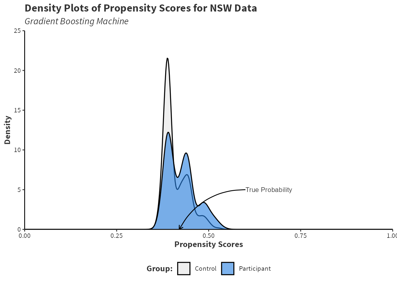
Figure 2.3 shows the propensity scores resulting from a GBM model using the gbm package on the NSW data provides. A GBM is a notable performance improvement to random forest and bagging shown in Figure 2.1. Recall that a “better” model would predict probabilities near to \(42\%\) as this is the treatment/control share in the randomised NSW data.
# Create Figure 2.3set.seed(88)library(gbm)nsw_gbm <-gbm(treat ~ age + educ + re75 + black + hisp + degree + marr, distribution ="bernoulli", data = nsw_data, n.trees =10000, shrinkage =0.0001)boosted_preds <-predict(nsw_gbm, type ="response")plot_pmachines(boosted_preds, "Gradient Boosting Machine") +scale_y_continuous(expand =expansion(0), limits =c(0, 25)) +annotate(geom ="curve", x =0.6, y =5, xend =0.42, yend =0, curvature = .3, arrow =arrow(length =unit(2, "mm"))) +annotate(geom ="text", x =0.6, y =5, label ="True Probability", hjust ="left", color ="#333333", size =3) +labs(title ="Density Plots of Propensity Scores for NSW Data") + custom_ggplot_theme
Figure 2.3: Density estimates of the propensity scores for control and participant groups in the National Supported Work programme using the gbm package with distribution = "bernoulli", data = nsw_data, n.trees = 10000, and shrinkage = 0.0001.
2.2.4 Overfitting
Overfitting is a common concern when fitting machine learning models, as models can capture noise and random variations in the training data. An overfit model typically shows excellent performance on the training data but will perform poorly on new, unseen data because it cannot generalise beyond the specific patterns of the training set. For instance, consider a machine learning algorithm used by a bank for fraud detection. In this scenario, an overfit model would struggle to classify transactions correctly as it has learned the noise and specific variation in the training data rather than the underlying patterns of fraud. Cross validation or test/train splitting can prevent overfitting to ensure a model can generalise to unseen data.
However, the model is not required to generalise a propensity score model as different datasets will have a different model. Instead, the emphasis of predicting propensity scores is to create balance in the data. A model is effective if it balances covariates between groups, even if it is overfit in a conventional sense.
Note 2.6: Overfitting in Logistic Regression
There is limited research on how overfitting a logistic regression model affects estimating treatment effects. In logistic regression, overfitting occurs when there are too many parameters and so the maximisation of the log-likelihood function is difficult because of noise. One study that investigates overfitting in this context is Schuster, Lowe, and Platt (2016), who suggest a general rule that the number of observations per parameter should be between \(10\) and \(20\). When overfitting occurs, the variance of the estimated treatment effect increases because noise amplifies the magnitude of the coefficients, resulting in a small bias towards \(0\) or \(1\) because of properties of the logit function. Specifically, when using (non-augmented) propensity score weighting, the estimate of the treatment effect will have high variance as propensity scores close to \(0\) or \(1\) receive artificially inflated weighting.
Lee, Lessler, and Stuart (2010) simulates a comparison of machine learning methods for propensity score prediction and finds that an overfit CART model performs better than a pruned CART model in terms of balance and treatment effect estimation bias. While not conclusive, this suggests that conventionally overfit trees are appropriate and potentially beneficial for propensity score modelling.
If overfitting was to occur, this could be interpreted as balance between groups getting worse decreases with a higher model complexity. Although various software packages use a stopping rule to prevent this. As conventional advice states, creating balance should be the aim of estimating propensity scores with overfitting being a minor concern.
2.3 Comparison of Machine Learning Algorithms: Simulation Results
Tu (2019) compares logistic regression, boosting, bagging, and random forests across different sample sizes, conditions of linearity and additivity, and treatment effect strengths. Boosting achieves the lowest bias ATE estimate in most scenarios and the lowest mean square error in all scenarios. Bagging ensembles and random forests perform poorly in both ATE estimate bias and MSE. The author notes that poor performance in bagging ensembles is likely due to correlated trees in the ensemble, leading to divergence bias. Random forests perform significantly better than bagging but both methods performed worse than boosting or logistic regression.
Despite poor theoretical properties as a probability machine, Lee, Lessler, and Stuart (2010) find that bagging results in the lowest standard error across many datasets.3 This result is not surprising given that the bagging ensembles are trained on bootstrapped datasets, leading to lower variance and standard error. Although, this advantage is not likely of practical interest given that the small performance gain in standard error is at the expense of a considerable increase of bias.
Additionally, Lee, Lessler, and Stuart (2010) finds that logistic regression performs well in simple data structures with comparable bias to boosting and random forest, but with larger standard errors. In complex data structures, boosting shows low bias and outperforms logistic regression while maintaining low standard errors. Consequently, the study concludes that boosted CART achieves the best \(95\%\) coverage in all simulation scenarios, with \(98.6\%\) coverage.4
Cannas and Arpino (2019) also undergo a simulation study to assess machine learning methods for propensity score prediction. They compare logistic regression, CART, bagging ensembles, random forest, boosting, neural networks, and naive bayes and find that random forest, neural networks, and logistic regression perform the best. Notably, the simulation design only performs hyperparameter tuning for CART, random forest, and neural networks but not either of their boosting implementation.5 This is a weakness of their study design and thus their findings may be more informative of the relative performance of tuned versus untuned models. Although, the finding that random forest performs well when tuned is significant.
Goller et al. (2020) adds diversity to the simulation study literature by exploring an economics context, experimenting with imbalances between treated and control observations, and incorporating LASSO and probit models.67 Probit regression achieves the best covariate balance, with LASSO also performing well. In contrast, the random forest model performs poorly, showing imbalance statistics with several orders of magnitude higher than those of probit or LASSO. To perform feature selection, a probit model with many interactions and polynomial terms is specified, and a LASSO penalty shrinks covariate coefficients to zero. Probit regression stands out for its superior covariate balance, while LASSO also delivers satisfactory results. The random forest model underperforms with significantly higher imbalance statistics compared to probit and LASSO.
Based on a review of the literature, the findings can be distilled into five important points:
Probability machines can predict propensity scores with excellent performance and their implementation should be considered in most scenarios. Although, a logistic regression approach may be preferred because of simplicity while still providing adequate performance in simple data structures.
In cases of non-linearity or non-additivity in the data, probability machines often achieve better covariate balance and lower bias of treatment effect estimates than logistic regression. This is significant as propensity scores are frequently used in observational studies with complex data structures (Rosenbaum and Rubin 1983).
Bagging ensembles perform poorly, a finding replicated across multiple studies.
Random forests can perform excellently when hyperparameters are satisfactorily tuned.
Further research should consider parametric methods with LASSO, Ridge, or Elastic Net penalties to assist in feature selection. Simulation study evidence for predicting propensity scores is limited despite attractive properties of these methods.
A tuned GBM stands out with strong theoretical support, excellent simulation performance, and superior software implementation and documentation. Specifically, this GBM will use the Bernoulli deviance as a loss function due to theoretical benefits. Implementations of GBMs such as AdaBoost.M1 have no simulation study evidence.
A good practical approach seems to be a trial-and-error approach of fitting multiple model specifications, then considering covariate balance for each model.
Austin, Peter. 2011. “An introduction to propensity score methods for reducing the effects of confounding in observational studies.”Multivariate Behavioral Research 46 (3): 399–424. https://doi.org/10.1080/00273171.2011.568786.
Austin, Peter C. 2008. “A critical appraisal of propensity-score matching in the medical literature between 1996 and 2003.”Statistics in Medicine 27 (April): 2037–49. https://doi.org/10.1002/sim.3150.
Bader-El-Den, Mohammed, Eleman Teitei, and Todd Perry. 2019. “Biased Random Forest for Dealing with the Class Imbalance Problem.”IEEE Transactions on Neural Networks and Learning Systems 30 (7): 2163–72. https://doi.org/10.1109/TNNLS.2018.2878400.
Breiman, Leo, Jerome H Friedman, Richard A Olshen, and Charles Stone. 1984. Classification and Regression Trees. Chapman; Hall/CRC. https://doi.org/10.1201/9781315139470.
Brookhart, M. Alan, Sebastian Schneeweiss, Kenneth J. Rothman, Robert J. Glynn, Jerry Avorn, and Til Stürmer. 2006. “Variable selection for propensity score models.”American Journal of Epidemiology 163 (12): 1149–56. https://doi.org/10.1093/aje/kwj149.
Cannas, Massimo, and Bruno Arpino. 2019. “A comparison of machine learning algorithms and covariate balance measures for propensity score matching and weighting.”Biometrical Journal 61 (4): 1049–72. https://doi.org/10.1002/bimj.201800132.
Cunningham, Scott. 2021. “Matching and Subclassification.” In Causal Inference: The Mixtape, 175–240. Yale University Press. https://doi.org/10.2307/j.ctv1c29t27.8.
Ferri-García, Ramón, and María Del Mar Rueda. 2020. “Propensity score adjustment using machine learning classification algorithms to control selection bias in online surveys.”PLoS ONE 15 (4): 1–19. https://doi.org/10.1371/journal.pone.0231500.
Friedman, Jerome H. 2001. “Greedy Function Approximation: A Gradient Boosting Machine.”The Annals of Statistics 29 (5): 1189–1232. https://www.jstor.org/stable/2699986.
Goller, Daniel, Michael Lechner, Andreas Moczall, and Joachim Wolff. 2020. “Does the estimation of the propensity score by machine learning improve matching estimation? The case of Germany’s programmes for long term unemployed.”Labour Economics 65 (March). https://doi.org/10.1016/j.labeco.2020.101855.
Heinrich, Carolyn, Alessandro Maffioli, and Gonzalo Vázquez. 2010. “A Primer for Applying Propensity-Score Matching.” August. http://dx.doi.org/10.18235/0008567.
King, Gary, and Richard Nielsen. 2019. “Why Propensity Scores Should Not Be Used for Matching.”Political Analysis 27 (4): 435–54. https://doi.org/10.1017/pan.2019.11.
Lee, Brian K., Justin Lessler, and Elizabeth A. Stuart. 2010. “Improving propensity score weighting using machine learning.”Statistics in Medicine 29: 337–46. https://doi.org/10.1002/sim.3782.
McCaffrey, Daniel F., Greg Ridgeway, and Andrew R. Morral. 2004. “Propensity score estimation with boosted regression for evaluating causal effects in observational studies.”Psychological Methods 9 (4): 403–25. https://doi.org/10.1037/1082-989X.9.4.403.
Olson, Matthew A., and Abraham J. Wyner. 2018. “Making Sense of Random Forest Probabilities: a Kernel Perspective,” 1–35. http://arxiv.org/abs/1812.05792.
Rosenbaum, Paul R., and Donald B. Rubin. 1983. “The central role of the propensity score in observational studies for causal effects.”Biometrika 70 (1): 41–55. https://doi.org/10.1017/CBO9780511810725.016.
Schuster, Tibor, Wilfrid Kouokam Lowe, and Robert W. Platt. 2016. “Propensity score model overfitting led to inflated variance of estimated odds ratios.”Journal of Clinical Epidemiology 80: 97–106. https://doi.org/10.1016/j.jclinepi.2016.05.017.
Setoguchi, Soko, Sebastian Schneeweiss, Alan M. Brookhart, Robert J. Glynn, and Francis E. Cook. 2008. “Evaluating uses of data mining techniques in propensity score estimation: a simulation study.”Pharmacoepidemiology and Drug Safety 17 (March): 546–55. https://doi.org/10.1002/pds.
Smith, Jeffrey A., and Petra E. Todd. 2005. Does matching overcome LaLonde’s critique of nonexperimental estimators? Vol. 125. 1-2 SPEC. ISS. https://doi.org/10.1016/j.jeconom.2004.04.011.
Tibshirani, Robert. 1996. “Regression Shrinkage and Selection via the Lasso.”Journal of the Royal Statistical Society 58 (1): 267–88. https://www.jstor.org/stable/2346178.
Tu, Chunhao. 2019. “Comparison of various machine learning algorithms for estimating generalized propensity score.”Journal of Statistical Computation and Simulation 89 (4): 708–19. https://doi.org/10.1080/00949655.2019.1571059.
IPW is also commonly known as inverse probability of treatment weighting (IPTW). IPTW uses propensity scores and can equally be called IPW.↩︎
Note that tuning \(mtry\) for the mean square of probability prediction is only possible by design of the simulation study and is not possible in applications, as the true probability is unknown.↩︎
In this case, the standard error is the dispersion of the standardised mean difference (effect size) across 1000 simulated datasets.↩︎
In this context, the coverage is the proportion of times that the true treatment effect is within the \(95\%\) confidence interval across the number of simulations. This author implements \(1000\) simulations of each scenario.↩︎
Cannas and Arpino (2019) provide a replication package for their simulation study online and their hyperparameter tuning is process transparent. The authors fit two GBMs using the twang and gbm package in R. The hyperparameter values provided to these untuned boosting models are contrary to heuristics and may lead boosting to perform poorly regardless of theoretical benefits discussed in Section 2.2.3.↩︎
Goller et al. (2020) calculates the bias of the treatment effect using the average of the estimates from logistic regression, random forest, and LASSO models as the true treatment effect. Thus, the covariate balance table offers a clearer view of each method’s performance.↩︎
Tibshirani (1996) introduces LASSO regularization, short for Least Absolute Shrinkage and Selection Operator, is a technique used in linear regression to prevent overfitting by penalising the absolute size of the coefficients. It adds a penalty term to the ordinary least squares objective function, meaning that some coefficients may “shrink” to zero.↩︎
Source Code
# Propensity Scores and Machine Learning {#sec-propensity}```{r}#| include: falseload(file ="globals.RData")```## A Conventional Approach: Propensity Scores and BalanceIn a randomised control trial (RCT), researchers believe treatment and control groups are similar because of randomisation. In this case, the similar groups are compatible and should not have systematic differences. In observational data, the exposure to a treatment is unlikely to be random, implying there may be systematic differences between groups. Systematic differences refer to consistent variations or disparities between groups in the study. These differences are not due to random chance but rather indicate a pattern or trend, perhaps due to selection-bias. As groups are not comparable, @eq-ate-estimate leads to a biased estimate of the treatment effect.For example, consider the causal question: *"How much does obtaining a bachelors degree increase lifetime earnings?"*. Individuals who complete a bachelor's degree are not selected at random for university programs (treatment) and may have different observable attributes than those who do not attend a university (control). Perhaps those who attend university have higher academic abilities, higher motivation, or grew up with parents with higher income. Because of these systematic group covariate differences, a simple comparison of mean income could lead to attributing university attendance as the *cause* of higher incomes when the effect is confounded by the differences in covariates between groups. In this example, the confounding covariates are academic ability, motivation, and parental income that impact the probability of someone obtaining a bachelors degree. This discussion introduces the idea of *covariate balance* which is a key concept behind underlying propensity score methods.::: {#nte-balance-intution .callout-note title="What is Covariate Balance"}Covariate balance is the idea that covariates are approximately equivalent across treatment and control groups. If the distribution of each covariate is the same across each group, then the covariates are *balanced* and a meaningful comparison between groups can be made. Equally, similar covariates across groups implies exchangability as the two groups should be similar (thus can be exchanged). There is a conceptual link between covariate balance, unconfoundedness, and exchangeability meaning that @eq-independence is satisfied when covariates are balanced. :::In the bachelor's degree example, suppose that comparable treatment and control individuals are matched together to create balanced pairs. Between these pairs, covariates are balanced such as the same academic ability, motivation, parental income, geographic residence etc. The covariates are said to be *conditioned on* by matching individuals on these covariates. Comparing the balanced matched pairs should result in a robust estimate of a bachelors degree's impact on earnings because the individuals are exchangeable and satisfy @eq-conditional-independence. However, practically this matching is difficult to perform as exact matches cannot be made as the number of covariates increases. For example, finding two people with the same gender is simple but finding two people with the same gender, age, education, income, motivation, location, experience, and race is nearly impossible. Thus, there is a *dimensionality* problem as the dimension of the number of covariates increases.@Rosenbaum1983 offer a valuable tool for analysing observational data called the propensity score. The propensity score is the probability of treatment assignment conditioned on observed covariates. Essentially, the propensity score reduces the dimension of the number of covariates to a single dimension to avoid the dimensionality problem. Let the propensity score be denoted as $e(X)$ and be expressed as:$$e(X)=P(T=1|X=x).$$ {#eq-pscore}A prediction of the conditional probability of treatment on covariates is a good summary of the covariate's effect on receiving the treatment. The covariate imbalance between bachelors degrees and controls arose from people self-selecting themselves into a bachelors degree programme because of these covariates. For example, people with higher motivation and academic ability are more likely to go to university. If it is the covariates that impact the probability of going to university, then a prediction of the probability of going to university based on these covariates should summarise the covariate effects. It is hoped that conditioning on this propensity score should balance the data and meet the conditional independence assumption stated in @eq-conditional-independence. There are many sources that offer a comprehensive guide to propensity score methods such as [@C5Mixtape2021, Chapter 4] who provides applications and coded examples in R, Python, and Stata.::: {#nte-balance-pscore .callout-note title="Balance and Propensity Scores"}Note that an RCT will satisfy @eq-independence as randomisation implies the potential outcomes are independent of the treatment assignment. Propensity score methods aim to satisfy @eq-conditional-independence as the potential outcomes are independent of the treatment status conditioned on some covariates. Thus, $Y(1), Y(0) \perp \!\!\! \perp T\mid X$ is satisfied by $Y(1), Y(0) \perp \!\!\! \perp T\mid \widehat{e(X)}$. Conditioning on the propensity score aims to replicate an RCT in observational data by balancing covariates between groups. When observations are conditioned on their propensity score, differences in outcomes can be confidently attributed to the treatment itself, rather than to pre-existing differences in covariates.:::Two common methods that use propensity scores are propensity score matching (PSM) and inverse propensity weighting (IPW).[^ipw] PSM creates matched sets with similar propensity scores. IPW creates a balanced pseudo-population, where observations are weighted on the inverse of the propensity score. The pseudo-population is created by up-weighting observations with a low propensity score and down-weighting observations with a high propensity score.[^ipw]: IPW is also commonly known as inverse probability of treatment weighting (IPTW). IPTW uses propensity scores and can equally be called IPW. At a high level, the conditioned property of the propensity score is translated into a model by using PSM or IPW. @King2019 provide a notable criticism of propensity score matching, which is a very interesting read. In the following examples, IPW is used due to theoretical advantages and ease of software implementation.### Assessing balance {#sec-assessing-balance}Balance assessment is an important step to ensure that conditioning on the propensity score has been successful. A commonly recommended measure of covariate balance is the standardised mean difference or **SMD**. This is the difference in the mean of each covariate between treatment groups standardised by a standardization factor so that it is on the same scale for all covariates. SMDs close to zero indicate good balance. @Austin2011 notes that $0.1$ is a common *threshold* for determining if a variable is balanced. This threshold is a guideline to the approximate region that indicates a covariate is balanced and should not be interpreted as a binary rule. Additionally, a variance ratio below *2* is generally acceptable. For brevity, my analysis only considers the SMD. ### Propensity Score Modelling with Logistic RegressionA conventional propensity score model uses logistic regression to predict a probability between $0$ and $1$. Models may be specified to include interaction terms and polynomial terms to capture complex trends in the data. There are a range of approaches for specifying a propensity score model, but the process is a heuristically driven art rather than science. [see @Brookhart2006; @Heinrich2010]. One suggestion is to include two-way interaction terms between covariates and squared terms and then remove terms which are not statistically significant. Notably, many researchers do not discuss the specification of propensity models in their papers. @Austin2008 reviews $47$ papers that use propensity scores and find few perform adequate model selection, assess balance, or apply correct statistical tests.It is important to note that the true propensity score is never observable. A propensity score that is close to the theoretically true probability is well calibrated. Poorly calibrated propensity scores may result in poor balance and biased estimation of the treatment effect. Propensity scores may be poorly calibrated as covariates may be omitted by error, poorly measured, or be unobservable. Logistic regression may not predict calibrated scores if the true relationship is non-linear or involves complex interactions between covariates. Another important note is that the propensity model itself does not have an informative *causal* interpretation. In logistic regression, the coefficients are the log-odds of the treatment assignment for each variable which is not informative of the desired estimand.The first application of machine learning in causal inference was to predict propensity scores. Despite this, logistic regression still appears to be the most common model for predicting propensity scores.## Probability Machines: Probability Theory and Machine LearningSupervised machine learning usually focuses on classifying observations into groups, or predicting continuous outcomes. Probability prediction is a hybrid of these tasks, aiming to predict the continuous probability an observation belongs to a certain class. Machine learning methods that predict probabilities are sometimes called probability machines. Probability machines are valuable in applications requiring calibrated probability predictions. For example, probability machines can predict loan defaults or other adverse events in finance. In marketing, they estimate the likelihood of customer response to a campaign. Gamblers and bettors want robust probability predictions to enhance their betting strategies. Probability machines can be applied wherever calibrated probability predictions are needed.Probability machines offer many advantages over parametric methods like logistic regression:1. **Improved Calibration**: Probability machines often provide better-calibrated predictions by capturing complex data relationships.2. **Flexible Modelling**: Unlike parametric methods like logistic regression, probability machines don't rely on assumptions of additivity or linearity, allowing them to model intricate relationships that parametric models miss.3. **Efficient Feature Selection**: These machines automatically select features, making them ideal for high-dimensional datasets where manual selection is impractical.4. **Handling Missing Data**: Probability machines handle missing data robustly, minimizing the need for extensive data reprocessing and imputation.5. **Simplified Data Exploration**: By exploring complex data structures in a data-driven way, probability machines simplify model specification. For instance, tree-based models remain unaffected by adding squared or interaction terms, streamlining the modeling process.In causal inference, probability machines can predict better calibrated propensity scores and better estimate treatment effects. This discussion aims to clarify the use of probability machines in causal inference given the unique requirements of propensity score specification. Probability machines are theoretically complex and there are unanswered questions in this space.::: {#nte-cart .callout-note title="A Particularly Important Method: Classification and Regression Trees"}Moving forward, a particularly important model is the Classification and Regression Trees. @Breiman1984 introduces method, commonly known as CART, that partitions data according to a splitting criterion, resulting in an "if this, then that" interpretation. CART models are also widely known as a decision trees. The splits are recursive, meaning splits are applied upon previous splits, such as trees breaking into branches and then leaves. The splits are also *greedy* as each potential split only considers information available at that split instead of past or future splits. Each parent node is split to create two child nodes and the final nodes of a CART model are called terminal nodes. For example, when classifying pets into cats versus dogs, the first split might be*"if barks"* and the second is *"heavier than 5 kg"*. The tree says *If it barks and is heavier than 5 kg, then it is a dog*.A single classification tree typically uses the Gini index to determine its splits. Each split aims to maximise node purity, meaning the nodes contain the highest possible proportion of one class. The Gini index measures impurity, with lower Gini values indicating higher purity. Intuitively, the aim of a classification tree’s loss function is to minimise the misclassification rate of observations. By selecting splits that reduce the Gini index, the tree minimises classification error and increases accuracy.:::### Choice of Loss Function and Probability PredictionThe loss function measures the difference between a model's predictions and the actual target values, serving as a measure of a model's performance. Different loss functions influence a model's behaviour so the choice of loss function is important. Classification models predict the category that each observation belongs to not the probability of each class. For instance, in fraud detection, banks use classifiers to distinguish between fraudulent and routine transactions. Many classification loss functions minimise classification errors and improve accuracy as this results in the best classification. A loss function like the Gini index is effective for classification problems but it is unclear if this applies to probability problems. In other words, minimizing misclassification error may not lead to accurate probability predictions.At a high level, to classify an observation, $x_i$ as an $A$ or $B$, a model needs to determine if $\Pr(x_i=A)$ is less than or greater than $0.5$. If $\widehat{\Pr}(x_i=A) > 0.5$, then it is more likely to be an $A$ and if $\widehat{\Pr}(x_i=A) <0.5$ then it is more likely to be a $B$. Thus, if $x_i$ is an $A$, it is trivial if $\widehat{\Pr}(x_i=A)$ is $0.51$ or $0.99$ as this makes no difference to the classification as an $A$. But the difference between $\widehat{\Pr}(x_i=A) = 0.51$ and $0.99$ is extreme for a probability machine. It is important to understand that classification models are optimised for classification accuracy rather than probability prediction. This distinction affects the performance of ensemble methods like random forests or bagging ensembles that use classification trees for probability prediction.### Bagging and Random Forest as Probability Machines {#sec-bagg-rf-probmachines}::: {#nte-ensemble .callout-note title="A Quick Note on Ensemble Learning"}Ensemble learning refers to a general framework of machine learning that combines multiple simple models to create a better overall model. The philosophy behind ensemble learning is rooted in the wisdom of crowds principle, where the collective decisions from multiple models often outperform that of individual models. Often, ensemble learning methods use multiple CART models.Bagging ensembles, random forests, and gradient boosting machines are all machine learning methods that combine CART models and are all examples of ensemble learning algorithms. These methods are introduced in the following discussion.:::Consider an ensemble method called the *lazy ensemble* that combines multiple CART trees. Each tree is fitted on the same data without any cross validation. In this ensemble, class probabilities are determined through a *vote count* method. Within the lazy ensemble, each tree makes a class prediction based on the majority class in a terminal node. For instance, if $x_i$ lies in a terminal node where $80\%$ of the observations are classified as an $A$, that *individual tree* will classify $x_i$ as $A$. The ensemble's *overall prediction* for $x_i$ is derived from the proportion of trees that classify $x_i$ as $A$ or $B$. Thus, the ensemble *counts votes* for each class across the ensemble. Let $T$ be the total number of trees and $b_t$ be the $t$-th tree in the ensemble. Let $\mathbb{I}(b_t(x_i) = A)$ be the indicator function that returns $1$ when $b_t$ predicts that observation $x_i$ belongs to class $A$. The probability of class $A$ for observation $x_i$ is calculated as:$$\widehat{\Pr}(x_i = A) = \frac{1}{T} \sum_{t=1}^{T} \mathbb{I}(b_t(x_i) = A). $$ {#eq-ensemble-vote-method}@Olson2018 note bias towards predictions of $0$ or $1$ when trees in an ensemble framework are highly correlated and a vote count method is used. In the lazy ensemble, each tree is identical and perfectly correlated implying that each tree will make the the same class prediction for each $x_i$. For such an ensemble, the predicted probabilities will will be exactly $0$ or $1$ using a vote count. Of course a lazy ensemble of identical trees would never be used but the intuition still applies in the real world where ensembles may have some degree of correlation. The larger the correlation, the more the probability predictions will exhibit a *divergence bias* towards $0$ and $1$. Notably, divergence bias is not problematic in classification applications, as a larger number of trees correctly classifying the observation is encouraging.To reduce tree correlation and improve upon the lazy ensemble, a bagging ensemble [see @Breiman1996] trains each tree on a randomly selected bootstrapped sample of the data. Random forests [see @Breiman2001] further reduce tree correlation by considering a random number of variables at each split, commonly referred to as $mtry$ in software implementations. When $mtry$ is equal to to number of predictors, the model considers all variables at each split and the random forest is equal to a bagging ensemble. Note that these ensemble methods typically use a *vote count method* in the same way as the lazy ensemble. A lower $mtry$ should reduce the correlation between trees and decrease divergence bias as the structure of the tree is modified by the selected variables at each split. However, a lower $mtry$ also introduces other theoretical problems.Consider the scenario where the binary outcome (treatment and control) of the ensemble is strongly related to a single predictor and weakly related to other noisy predictors. If $mtry$ is low then each split may not consider the strong predictor and more commonly splits on weak or noisy predictors. Each predictor has a chance of $\frac{mtry}{\text{number of predictors}}$ of selection at each split implying a lower $mtry$ decreases the chance of a splitting on the strong predictor. Splits on the weak or noisy predictors may not result in a meaningful increase in node purity and successive splits may result in impure terminal nodes that poorly predict the class of $x_i$ in each tree. Such an ensemble may have highly unstable probability predictions. Additionally, consider there is a class imbalance and the majority of observations are classified as $A$ not $B.$ The terminal nodes of each tree within an ensemble are more likely to contain the majority class. Consequently, there is a *majority class bias* as each tree in the ensemble is more likely to misclassifying an observation as an $A$ because the terminal nodes have a higher proportion of $A$ due to the higher proportion of $A$'s in the data overall.::: {#nte-class-imbalance .callout-note title="Class Imbalance and Machine Learning"}When there is a difference in the number of observations in each class, this is called class imbalance. It is important to note that majority class bias exists in conventional machine learning classification tasks. Bagging ensembles and random forest are well known to be sensitive to class imbalance meaning that class predictions are biased towards the majority [see @Bader2019].However, the class imbalance problem is particularly notable when predicting probabilities. The probability prediction from a vote count method is very sensitive to a change in the votes from each tree. Suppose that balanced data results in $80/100$ trees classifying $B$ as $B$ and imbalanced data (more $A$ than $B$) reduces correct classifications of $B$ to $60/100$. This results in a $20\%$ margin of error in probability estimates but the classification remains as $B$.:::Individually, a low $mtry$ can lead to unstable probability predictions and class imbalance can create bias towards the majority class. But probability machines are particularly effected when there is both a low $mtry$ *and* class imbalance. Because successive noisy splits (relating to a low $mtry$) result in impure child nodes, the effects of majority class bias are exaggerated. Without the ability to separate the classes, the majority class will dominate terminal nodes. If the ensemble was able to split on informative covariates each time ($mtry$ is higher), then it should still be able to create pure splits even when there is some class imbalance. In other words, if there is a small class imbalance, reducing $mtry$ may reveal majority class bias not visible at higher $mtry$'s. Equally, if there is low $mtry$, then even a small class imbalance can lead to majority class bias. As a general philosophy, ensemble learning methods based on classification trees are poor at predicting probabilities. If $x_i$ has a known membership of $A$, and an unknown $\Pr_{\text{true}}(x_i=A) = 0.6$, the ensemble might classify $x_i$ correctly $90\%$ of the time leading to $\widehat{\Pr}(x_i=A) = 0.9$. As a probability machine, the ensemble has overestimated the probability by $30\%$ even though a $90\%$ classification accuracy is excellent. To predict $\Pr_{\text{true}}(x_i=A) = 0.6$, an ensemble needs to incorrectly classify $x_i$ in $40\%$ of its trees. However, bagging ensembles and random forests are designed to maximise classification accuracy and there is no incentive for the model to intentionally achieve a specific misclassification rate that aligns with the true probability.To exemplify these theoretical points, the National Supported Work (NSW) programme is a commonly discussed dataset in causal inference. The data results from a randomised controlled trial with $445$ total participants, $185$ in the program group, and $260$ in the control group, so the true probability of treatment for each individual can be calculated as $185/445=0.42$ or $42\%$. Further information about this data is found in @sec-datasets. Randomisation should ensure that the probability of treatment is independent of the predictors and so all predictors should be noisy or weak. Although @fig-rf-varimp and @tbl-combined-btab suggest some covariates do have a greater impact on the probability of participating in the programme, which echoes research by @Smith2005 who suggest randomisation is imperfect in the NSW dataset. Thus, the "best" calibrated probability model will have a distribution centred near $0.42$ with some noise due to imperfect randomisation.@fig-rf-theory-demo shows both divergence bias and majority class bias using `randomForest()` to fit both the random forest and bagging ensemble. Recall that a bagging ensemble is a random forest model when $mtry$ is equal to the number of predictors and so specifying `mtry = 7` in the `randomForest()` function fits a bagging ensemble. Additionally, logistic regression using the `glm()` function provides a meaningful comparison.```{r }#| dev: "ragg_png"#| fig-height: 8#| label: fig-rf-theory-demo#| code-fold: true#| echo: !expr "knitr::is_html_output()"#| code-summary: "Code: Create [Figure 2.1](fig-rf-theory-demo)" #| fig-cap: "Compares the density estimates of the propensity scores for control and participant groups in the National Supported Work programme. `randomForest()` fits a random forest with `mtry = 1` and bagging ensemble with `mtry = 7`. The default values of `ntree = 500` and `nodesize = 1` are used. A logistic regression model is included for a comparison."# Create Figure 2.1library(randomForest)library(patchwork)library(ggplot2)library(ragg)set.seed(88)nsw_formula <- as.formula(as.factor(treat) ~ age + educ + re75 + black + hisp + degree + marr)logit_preds <- glm(nsw_formula, data = nsw_data, family = binomial())$fitted.values rf_mtry1_preds <- predict(randomForest(nsw_formula, mtry = 1, data = nsw_data), newdata = nsw_data, type = "prob")[, 2]bagging_model <- randomForest(nsw_formula, mtry = 7, importance = TRUE, data = nsw_data)bagged_preds <- predict(bagging_model, newdata = nsw_data, type = "prob")[, 2]plot_pmachines <- function(pscores, plot_subtitle) { ggplot(nsw_data, aes(x = pscores, fill = factor(treat))) + geom_density(alpha = 0.6, linewidth = 0.6) + scale_fill_manual(values = c("#e5e5e5", "#2780e3"), labels = c("Control", "Participant")) + labs(subtitle = plot_subtitle, x = "Propensity Scores", y = "Density", fill = "Group:") + scale_x_continuous(expand = expansion(0), limits = c(0,1)) + scale_y_continuous(expand = expansion(0), limits = c(0,10)) + custom_ggplot_theme}p1 <- plot_pmachines(logit_preds, "Logistic Regression") + xlab(NULL) + theme(legend.position = "none") + annotate(geom = "curve", x = 0.6, y = 5, xend = 0.42, yend = 0, curvature = .3, arrow = arrow(length = unit(2, "mm"))) + annotate(geom = "text", x = 0.6, y = 5, label = "True Probability", hjust = "left", color = "#333333", size = 3)p2 <- plot_pmachines(rf_mtry1_preds, "Random Forest (mtry = 1)") + xlab(NULL) + theme(legend.position = "none")p3 <- plot_pmachines(bagged_preds, "Bagging (Bootstrap Aggregation)")p1 / p2 / p3 + plot_annotation( title = "Density Plots of Propensity Scores for NSW Data", theme = custom_ggplot_theme)``````{r}#| dev: "ragg_png"#| label: fig-rf-varimp#| code-fold: true#| echo: !expr "knitr::is_html_output()"#| code-summary: "Code: Create [Figure 2.2](fig-rf-theory-demo)"#| fig-cap: "Compares the variable importance assigned to each variable from a bagging ensemble fitted on data from the National Supported Work programme. `randomForest()` fits a baggin ensemble with `mtry = 7` with default `ntree = 500` and `nodesize = 1`."# Create Figure 2.2library(ggplot2)library(tidyverse)imp <-as.data.frame(importance(bagging_model))imp <-cbind(vars =rownames(imp), imp)imp <- imp[order(imp$MeanDecreaseGini),]imp$vars <-factor(imp$vars, levels =unique(imp$vars))imp %>%pivot_longer(cols =matches("Mean")) %>%ggplot(aes(y = vars, x = value, fill = name)) +geom_bar(stat ="identity", width =0.8, show.legend =TRUE, position =position_dodge(width =0.8), color ="black", linewidth =0.6) +facet_grid(~factor(name, levels =c("MeanDecreaseGini", "MeanDecreaseAccuracy")), scales ="free_x") +scale_fill_manual(values =c("#e5e5e5", "#2780e3")) +scale_x_continuous(expand =expansion(c(0, 0.04))) +labs(title ="Variable Importance",x ="% Decrease if Variable is Omitted from Model", y ="Variable Name" ) + custom_ggplot_theme +theme(legend.position ="none")```@fig-rf-theory-demo shows the logistic regression model has identified a central tendency and most propensities are between $0.25$ and $0.75$ which roughly aligns with the true probability. The bagging ensemble has clear evidence of divergence and the majority of predictions are outside $0.25$ and $0.75$ which is likely related to tree correlation. For the random forest with $mtry=1$, a significant number of the treatment and control observations are centred near the control area ($T=0$) with a wide range of other predictions. Recall that the control group is the majority class. Reducing $mtry$ from $7$ to $1$ reveals the majority class bias reinforcing the theoretical discussion that a combination of low $mtry$ and class imbalance is especially troubling. The model over predicts the majority class and has unstable predictions otherwise. Both random forest and bagging ensembles have performed poorly. The tuning of $mtry$ faces double jeopardy and is another important area of discussion in probability machines. The selection of $mtry$ is typically carried out in with a classification loss function such as accuracy or out-of-bag error. @Olson2018 compares tuning $mtry$ measured by classification accuracy and mean square error of known simulation probabilities and finds that the optimal value of $mtry$ for classification differs from probability prediction.[^propensity-2] In other words, if a grid search finds that $mtry=3$ is optimal for a classification task, this does not imply that $mtry=3$ is optimal for predicting probabilities. Putting this together, $mtry$ is a double-edged sword, typically controlled with an imperfect method.[^propensity-2]: Note that tuning $mtry$ for the mean square of probability prediction is only possible by design of the simulation study and is not possible in applications, as the true probability is unknown.Random forests and bagging ensembles seem to be troubled as probability machines but this does not mean that bagging and random forest cannot perform well. In various simulation studies, they perform excellently as discussed in @sec-mlps-sims. Perhaps the nature of the data is informative for the potential success of a random forest or bagging ensemble.Heuristically, divergence bias and majority class bias will most affect a probability machine when there is considerable overlap of true probabilities between groups. Recall the meaning of *common support* and *overlap* from @sec-assumptions. If there is overlap and a central region of true probabilities, then the effects of divergence bias may be very pronounced. Similarly, common support may make it even harder to increase purity in child nodes, as the covariates will lack clear split points. When combined with weak predictors relating to a low $mtry$, the terminal nodes of each tree may be relatively impure leading to a majority class bias. Alternatively, if true probabilities exist near $0$ or $1$ and there is a clear separation of class, divergence bias may trivially effect probability estimation as the probabilities already exist in that region. If there is a clear separation of class, then weak predictors relating to a low $mtry$ may still create meaningful splits and pure terminal nodes. It is worth noting that propensity score methods require datasets with overlap to meet the assumptions required to determine causality.### Gradient Boosting Machines as Probability Machines {#sec-gbm}Moving beyond classification trees in random forests or bagging ensembles, @Friedman2001 introduced the *Gradient Boosting Machine* (GBM). A GBM sequentially constructs CART trees to correct errors made by previous trees. Employing a gradient descent process, each new tree is fit on the pseudo-residuals of the previous iteration. This means that with each iteration, the GBM takes a gradient step down the global loss function, incrementally minimizing the loss function to reach a minimum. A learning rate controls the contribution of each weak learner to the final model. By using a small learning rate, the machine learns slowly so that it can slowly descend the loss function. This allows for finer adjustments during the iterative process to better capture patterns in the data. GBMs can be generalised to many different applications by minimizing a different loss function which can be specified as any continuously differentiable function. For binary outcomes, a GBM employs multiple regression trees and a logistic function to transform regression predictions into probabilities. Specifically, the logistic function used is:$$\widehat{\Pr}(x_i=A) = \frac{1}{1 + \exp(-\text{model}(x_i))}.$$ {#eq-gbm-logit}This logistic function is the same as in logistic regression, so a GBM with a binary class is sometimes called boosted logistic regression. The ensemble aims to minimise the Bernoulli deviance, which is equivalent to maximizing the Bernoulli log-likelihood with logistic regression. Maximizing the log-likelihood ensures that the predicted probability distribution is as close as possible to the true probability distribution given the data. The full GBM model, $f_T(x)$ after $T$ iterations can be written as:$$f_T(x_i) = b_1(x_i) + \lambda \sum_{t=1}^{T} b_t(x_i).$$ {#eq-gbm-model}Inside a base tree, each split considers all variables and makes the most informative split to descend the loss function using gradient descent. GBMs utilise many weak learners, such as a regression tree with a single split called a regression stump. However, additional splits enable the model to capture interactions between terms, which may increase probability calibration in complex or high-dimensional datasets.By outputting probability predictions and avoiding the flaws of vote methods in other ensemble techniques, as well as allowing a probability distribution-based loss function optimal for probability prediction, GBMs stand out as a highly effective probability machine. Since GBMs predict probabilities from a logistic function, they avoid problems associated with a vote count method. The implementation and workflow to fit a GBM for propensity scores is discussed in @sec-gbm-tune-workflow.@fig-gbm-demo shows the propensity scores resulting from a GBM model using the `gbm` package on the NSW data provides. A GBM is a notable performance improvement to random forest and bagging shown in @fig-rf-theory-demo. Recall that a "better" model would predict probabilities near to $42\%$ as this is the treatment/control share in the randomised NSW data. ```{r}#| dev: "ragg_png"#| label: fig-gbm-demo#| code-fold: true#| echo: !expr "knitr::is_html_output()"#| code-summary: "Code: Create [Figure 2.3](fig-gbm-demo)"#| fig-cap: "Density estimates of the propensity scores for control and participant groups in the National Supported Work programme using the `gbm` package with `distribution = \"bernoulli\"`, `data = nsw_data`, `n.trees = 10000`, and `shrinkage = 0.0001`."# Create Figure 2.3set.seed(88)library(gbm)nsw_gbm <-gbm(treat ~ age + educ + re75 + black + hisp + degree + marr, distribution ="bernoulli", data = nsw_data, n.trees =10000, shrinkage =0.0001)boosted_preds <-predict(nsw_gbm, type ="response")plot_pmachines(boosted_preds, "Gradient Boosting Machine") +scale_y_continuous(expand =expansion(0), limits =c(0, 25)) +annotate(geom ="curve", x =0.6, y =5, xend =0.42, yend =0, curvature = .3, arrow =arrow(length =unit(2, "mm"))) +annotate(geom ="text", x =0.6, y =5, label ="True Probability", hjust ="left", color ="#333333", size =3) +labs(title ="Density Plots of Propensity Scores for NSW Data") + custom_ggplot_theme```### OverfittingOverfitting is a common concern when fitting machine learning models, as models can capture noise and random variations in the training data. An overfit model typically shows excellent performance on the training data but will perform poorly on new, unseen data because it cannot generalise beyond the specific patterns of the training set. For instance, consider a machine learning algorithm used by a bank for fraud detection. In this scenario, an overfit model would struggle to classify transactions correctly as it has learned the noise and specific variation in the training data rather than the underlying patterns of fraud. Cross validation or test/train splitting can prevent overfitting to ensure a model can generalise to unseen data.However, the model is not required to generalise a propensity score model as different datasets will have a different model. Instead, the emphasis of predicting propensity scores is to create balance in the data. A model is effective if it balances covariates between groups, even if it is overfit in a conventional sense.::: {#nte-overfit-logistic .callout-note title="Overfitting in Logistic Regression"}There is limited research on how overfitting a logistic regression model affects estimating treatment effects. In logistic regression, overfitting occurs when there are too many parameters and so the maximisation of the log-likelihood function is difficult because of noise. One study that investigates overfitting in this context is @Schuster2016, who suggest a general rule that the number of observations per parameter should be between $10$ and $20$. When overfitting occurs, the variance of the estimated treatment effect increases because noise amplifies the magnitude of the coefficients, resulting in a small bias towards $0$ or $1$ because of properties of the logit function. Specifically, when using (non-augmented) propensity score weighting, the estimate of the treatment effect will have high variance as propensity scores close to $0$ or $1$ receive artificially inflated weighting.:::@Lee2010 simulates a comparison of machine learning methods for propensity score prediction and finds that an overfit CART model performs better than a pruned CART model in terms of balance and treatment effect estimation bias. While not conclusive, this suggests that conventionally overfit trees are appropriate and potentially beneficial for propensity score modelling.If overfitting was to occur, this could be interpreted as balance between groups getting worse decreases with a higher model complexity. Although various software packages use a stopping rule to prevent this. As conventional advice states, creating balance should be the aim of estimating propensity scores with overfitting being a minor concern.## Comparison of Machine Learning Algorithms: Simulation Results {#sec-mlps-sims}A small body of simulation studies benchmarks probability machines for predicting propensity scores [see @McCaffrey2004; @Setoguchi2008; @Lee2010; @Cannas2019; @Tu2019; @Goller2020; @Ferri2020]. Although these studies tackle the same problem, differences in simulation design and model implementation lead to a diverse range of perspectives on this issue. This variety reflects the complexity of the propensity score prediction.@Tu2019 compares logistic regression, boosting, bagging, and random forests across different sample sizes, conditions of linearity and additivity, and treatment effect strengths. Boosting achieves the lowest bias ATE estimate in most scenarios and the lowest mean square error in all scenarios. Bagging ensembles and random forests perform poorly in both ATE estimate bias and MSE. The author notes that poor performance in bagging ensembles is likely due to correlated trees in the ensemble, leading to divergence bias. Random forests perform significantly better than bagging but both methods performed worse than boosting or logistic regression.Despite poor theoretical properties as a probability machine, @Lee2010 find that bagging results in the lowest standard error across many datasets.[^propensity-3] This result is not surprising given that the bagging ensembles are trained on bootstrapped datasets, leading to lower variance and standard error. Although, this advantage is not likely of practical interest given that the small performance gain in standard error is at the expense of a considerable increase of bias.[^propensity-3]: In this case, the standard error is the dispersion of the standardised mean difference (effect size) across 1000 simulated datasets.Additionally, @Lee2010 finds that logistic regression performs well in simple data structures with comparable bias to boosting and random forest, but with larger standard errors. In complex data structures, boosting shows low bias and outperforms logistic regression while maintaining low standard errors. Consequently, the study concludes that boosted CART achieves the best $95\%$ coverage in all simulation scenarios, with $98.6\%$ coverage.[^propensity-4][^propensity-4]: In this context, the coverage is the proportion of times that the true treatment effect is within the $95\%$ confidence interval across the number of simulations. This author implements $1000$ simulations of each scenario.@Cannas2019 also undergo a simulation study to assess machine learning methods for propensity score prediction. They compare logistic regression, CART, bagging ensembles, random forest, boosting, neural networks, and naive bayes and find that random forest, neural networks, and logistic regression perform the best. Notably, the simulation design only performs hyperparameter tuning for CART, random forest, and neural networks but not either of their boosting implementation.[^propensity-5] This is a weakness of their study design and thus their findings may be more informative of the relative performance of tuned versus untuned models. Although, the finding that random forest performs well when tuned is significant.[^propensity-5]: @Cannas2019 provide a replication package for their simulation study online and their hyperparameter tuning is process transparent. The authors fit two GBMs using the `twang` and `gbm` package in R. The hyperparameter values provided to these untuned boosting models are contrary to heuristics and may lead boosting to perform poorly regardless of theoretical benefits discussed in @sec-gbm.@Goller2020 adds diversity to the simulation study literature by exploring an economics context, experimenting with imbalances between treated and control observations, and incorporating LASSO and probit models.[^propensity-6][^lasso] Probit regression achieves the best covariate balance, with LASSO also performing well. In contrast, the random forest model performs poorly, showing imbalance statistics with several orders of magnitude higher than those of probit or LASSO. To perform feature selection, a probit model with many interactions and polynomial terms is specified, and a LASSO penalty shrinks covariate coefficients to zero. Probit regression stands out for its superior covariate balance, while LASSO also delivers satisfactory results. The random forest model underperforms with significantly higher imbalance statistics compared to probit and LASSO.[^propensity-6]: @Goller2020 calculates the bias of the treatment effect using the average of the estimates from logistic regression, random forest, and LASSO models as the *true* treatment effect. Thus, the covariate balance table offers a clearer view of each method's performance.[^lasso]: @Tibshirani1996 introduces LASSO regularization, short for Least Absolute Shrinkage and Selection Operator, is a technique used in linear regression to prevent overfitting by penalising the absolute size of the coefficients. It adds a penalty term to the ordinary least squares objective function, meaning that some coefficients may "shrink" to zero.Based on a review of the literature, the findings can be distilled into five important points:1. Probability machines can predict propensity scores with excellent performance and their implementation should be considered in most scenarios. Although, a logistic regression approach may be preferred because of simplicity while still providing adequate performance in simple data structures.2. In cases of non-linearity or non-additivity in the data, probability machines often achieve better covariate balance and lower bias of treatment effect estimates than logistic regression. This is significant as propensity scores are frequently used in observational studies with complex data structures [@Rosenbaum1983].3. Bagging ensembles perform poorly, a finding replicated across multiple studies.4. Random forests can perform excellently when hyperparameters are satisfactorily tuned.5. Further research should consider parametric methods with LASSO, Ridge, or Elastic Net penalties to assist in feature selection. Simulation study evidence for predicting propensity scores is limited despite attractive properties of these methods.6. A tuned GBM stands out with strong theoretical support, excellent simulation performance, and superior software implementation and documentation. Specifically, this GBM will use the Bernoulli deviance as a loss function due to theoretical benefits. Implementations of GBMs such as AdaBoost.M1 have no simulation study evidence.7. A good practical approach seems to be a trial-and-error approach of fitting multiple model specifications, then considering covariate balance for each model.::: {.content-visible when-format="pdf"}## Code Provided for PDF Output```{r get-labels, echo = FALSE}labs = knitr::all_labels()labs = setdiff(labs, c("get-labels"))``````{r all-code, ref.label=labs, eval=FALSE}```:::```{r}#| include: falsesave.image(file ="globals.RData")```