3  Tutorial: Implimentation, Workflow, and Example with WeightIt andgbm in R

Based on Friedman (2001), the gbm package implements a Generalized Boosting Machine. Here, the “generalized” is because the package provides generalisations of the boosting framework to other distributions such as Bernoulli, Poisson, and Cox-proportional hazards partial likelihood of class probability predictions. Although this implementation very closely follows Friedman (2001) who introduced the gradient boosting machine. gbm also supports stochastic gradient boosting, which performs random bootstrap sampling for each tree using the bag.fraction parameter.

To fit and tune a GBM for propensity scores, wrapper packages facilitate optimal hyperparameter tuning for covariate balance. An effective approach involves fitting the model and computing balance statistics at each hyperparameter combination. Since the gbm package does not support this type of tuning, a wrapper package like WeightIt is necessary. WeightIt allows for hyperparameter tuning based on covariate balance and inverse propensity weighting (IPW). WeightIt supports hyperparameter turning of shrinkage, interaction.depth, and n.trees. Once the best model is identified, propensity scores are predicted inside WeightIt. These can be used inside WeightIt to perform IPW or extracted for other implementations. WeightIt also supports an offset meaning that logistic regression predictions are supplied to the GBM package.

Multiple sources, including package documentation and other research, suggest values for hyperparameters (see McCaffrey, Ridgeway, and Morral 2004; Ridgeway et al. 2024). A very low learning rate, such as \(0.01\) or \(0.0005\), allows a smooth descent of the loss function. The model should include a high number of trees, with \(10,000\) or \(20,000\) being a typical default value. While this may seem excessive, it is required when a low learning rate is used. A grid search process should consider many options including a very high number of trees and even though the optimal model may contain fewer trees. While GBMs often use shallow trees like stumps, allowing a few splits per tree can better model non-linearity and additivity. The WeightIt default allows for \(3\) splits. Based on anecdotal experience, \(1\) to \(5\) splits per tree is optimal, consistent with recommendations by McCaffrey, Ridgeway, and Morral (2004).

Another package, twang, proves functionality to tune the number of trees, but there are no inbuilt options for tuning of other hyperparameters and so accessory packages such as caret must be used. Although twang has other useful functionalities which users may wish to implement.

3.1 Hyperparameter Tuning and Workflow

The WeigthtIt package seems to have the best options for hyperparameter tuning and integration with a package for assessing balance called cobalt. The best information for this package can be found on this website or accessed with vignette("WeightIt") inside R after installation using install.packages("WeightIt").

A workflow for hyperparameter tuning in WeightIt may be completed as follows:

1. Specify the criterion option or measure of balance, which specifies the measure of the best model. The available measures are any balance measure that cobalt can compute. A simple option to choose may be the average standardised mean difference (SMD) across all covariates called sdm.mean or the smallest maximum SDM across covariates called sdm.max. It may be worthwhile to complete the tuning process with different tuning criteria.

2. Set the number of trees high. The package default is n.trees = 10000 for binary treatments, but this may be too small depending on the learning rate. Typically, it is best to increase the number of trees to ensure slow learners have the opportunity to reach their minimum criterion. There is no modelling downside to a larger number of trees other than computation time as the model will predict propensity scores with a smaller n.tree if optimal.

3. Specify the grid search for the depth of the tree called interaction.depth and the learning rate called shrinkage. These values can be specified using c() such as shrinkage = c(0.0005, 0.001, 0.05, 0.1, 0.2, 0.3) or as integers such as interaction.depth = 1:5. These particular values are heuristically selected suggestions of good starting values. Additionally, an offset can be considered by performing a grid search across offset = c(TRUE, FALSE).¹

4. The model is fit and a grid search is performed. The tune grid and balance statistics can be retrieved with my_weightit_object$info$best.tune.

5. The best model should be inspected and to determine if the initial grid is appropriate. If the selection of the best model is at the boundary of a grid search, then a new grid should be created and step 3 and 4 are repeated. For example, if the initial fit is completed with interaction.depth = 1:5 and the best fit is \(5\), then a new search can consider interaction.depth = 3:7 so that the local area around \(5\) can be searched.

6. Experiment with bag.fraction, which means each tree will consider a drawn proportion of observations equal to bag.fraction. Iteratively changing bag.fraction and assessing balance at each value should be practical. Consider \(0.5\), \(0.67\), and \(1\).

7. Assess balance of covariates and model fit. Covariate balance can be assessed with a balance table such as bal.tab() or visualised using love.plot() from cobalt.

8. The tuned model is stated and reported to allow replicable results. Balance tables are presented and discussed. Comparison to other methods of estimation if relevant.

9. Estimation and reporting of treatment effect.

3.2 Example: NSW Jobs Dataset Using R

For demonstration, propensity scores are estimated following the workflow discussed in Section 3.1 to estimate inverse propensity weights (IPW). The NSW jobs dataset arises from a randomised setting as described in Appendix A. Randomisation should eliminate structural differences between groups, but Rosenbaum and Rubin (1983) notes that randomisation only addresses structural balance and does not account for chance imbalance. To address this, propensity scores can mitigate any remaining chance imbalance, providing a more accurate estimate of the treatment effect. This example will include the fitting process of a GBM using WeightIt and a logistic regression model using glm(). Additionally, balance statistics will be computed leading to a robust estimate of the treatment effect.

Note 3.1: Inverse Probability of Treatment Weighting

Inverse probability of treatment weighting or inverse propensity weighting (IPW) adjusts for confounding in observational data by weighting individuals based on the inverse of their probability of receiving the treatment they actually got. This method creates a pseudo-population where treatment assignment is independent of observed covariates, similar to a randomised controlled trial. In this re-weighted population, the treatment and control groups should be have covariate balance, allowing for unbiased estimation of treatment effects. Essentially, IPW simulates random treatment assignment by rebalancing the sample, thereby eliminating confounding and enabling more accurate causal inferences.

3.2.1 Step 1-6: Model Fitting and Tuning

The glm() function will fit a conventional propensity score model with logistic regression in R. Logistic regression is performed by specifying the family to be the binomial(). Recall the nsw_formula is specified in Section 2.2.2.

nsw_logit_pmodel <- glm(nsw_formula, data = nsw_data,
1                        family=binomial())

2nsw_logit_pscores <- nsw_logit_pmodel$fitted.values

1

Fits a logistic regression model using the glm() function specified to be a logistic model with family=binomial() using the previously created nsw_formula.

2

Extracts the fitted values (propensity scores) from the model.

The weightit() function from the WeightIt package will perform IPW and assign a weight to each observation such that the pseudo-population should exhibit covariate balance. The model object will be called nsw_logit_weight.

library(WeightIt)
1nsw_logit_weight <- weightit(nsw_formula, data = nsw_data,
2                             ps = nsw_logit_pscores,
3                             estimand = "ATE")

1

Specifies the formula and data.

2

Provides weightit() with the propensity scores from the logistic regression function. Note that in practice this can be completed within the weightit() function with method = "glm". The separate estimation of the propensity scores is for illustrative purposes.

3

Specifies the estimand as the average treatment effect or ATE. For the purposes of demonstration, this is an arbitrary choice.

A GBM model for propensity scores can be specified using method = "gbm" inside the weightit() function. To ensure consistent results, running set.seed(88) will ensure each tree uses the same seed if bag.fraction less than \(1\). The model is fit using the heuristically suggested starting values. Note that this model may take approximately \(30\) second to fit as a grid search procedure is computationally intensive. Additionally, the best tuning specification is printed to assess if the initial tuning grid is appropriate.

set.seed(88)
1nsw_boosted_weight <- weightit(nsw_formula, data = nsw_data,
2                               method = "gbm",
                               estimand = "ATE",
                               shrinkage = c(0.0005, 0.001, 0.05, 
3                                             0.1, 0.2, 0.3),
                               interaction.depth = 1:5,
4                               bag.fraction = 1,
                               offset = c(TRUE, FALSE),
5                               criterion = "smd.mean",
                               n.trees = 10000)
6print(nsw_boosted_weight$info$best.tune)

1

Specifies the formula and data.

2

Specifies the propensity score prediction method to be a GBM and the estimand to the ATE.

3

Performs a grid search over these values of the learning rate and depth of tree.

4

Requires the model to use every observation in every tree, meaning the model will not perform stochastic gradient boosting. The function will will fit an offset and level GBM and select the specification with the best balance.

5

Defines the optimisation criteria to be the tune with the lowest average standardised mean difference (SMD). Additionally, the number of trees will be \(10000\) which is the package default.

6

Prints the tune details of the model with the best covariate balance.

  shrinkage interaction.depth distribution use.offset best.smd.mean best.tree
6       0.3                 1    bernoulli      FALSE    0.02253485      2392

The best balance across all tuning combinations yields an average SMD of \(0.023\) showing strong balance compared to the \(0.1\) threshold. Note averages can conceal extremes and a low average SMD does not mean all variables are balanced. A full balance table is presented in Section 3.2.2 accompanying a discussion of balance.

The best machine has a learning rate of \(0.3\) and contains \(2392\) decision stumps (trees with a depth of \(1\)). The learning rate is on the boundary of the initial tuning grid showing that the tuning grid should be re-specified to include values near to \(0.3\). A reduction in the depth of tree and number of trees will reduce computation time.

The new tune grid will consider shrinkage = c(0.25, 0.3, 0.35, 0.4, 0.45, 0.5) as this allows the GBM to consider values between \(0.2\) and \(0.3\) and above \(0.3\) which were missing in the previous grid.

# Additional weightit() GBM grid
set.seed(88)
nsw_boosted_weight2 <- weightit(nsw_formula, data = nsw_data, 
                               method="gbm",
                               estimand = "ATE", 
                               shrinkage= c(0.25, 0.3, 0.35, 0.4, 0.45, 0.5),
                               interaction.depth = 1:3,
                               bag.fraction = 1,
                               offset = c(TRUE, FALSE),
                               criterion = "smd.mean", 
                               n.trees = 5000)

print(nsw_boosted_weight2$info$best.tune)

   shrinkage interaction.depth distribution use.offset best.smd.mean best.tree
11      0.45                 2    bernoulli      FALSE    0.01965492        95

Comparing the two iterations, there is a reduction from \(0.022\) to \(0.02\) in the SMD. The optimal tuning values are towards the centre of the tuning grid, implying that an adequate search of the local area has been completed. The best machine has a learning rate of \(0.45\), a tree depth of \(2\), and \(95\) trees. The learning rate is higher than expected, but this also explains why fewer trees are optimal.

Plotting the relationship between the number of trees and the average SMD is informative for the behaviour of the machine. Additionally, Figure 3.1 shows the optimal number of trees is highly variable. If the learning rate is set to shrinkage = 0.05, then the best balance is not achieved until near to \(20,000\) trees.

# Create Figure 3.1
library(ggplot2)
library(patchwork)
low_shrinkage <- weightit(nsw_formula, data = nsw_data, 
                               method = "gbm",
                               estimand = "ATE", 
                               shrinkage = 0.05,
                               interaction.depth = 1,
                               offset = c(TRUE, FALSE),
                               criterion = "smd.mean", 
                               n.trees = 40000)

optimal_boost_plot <- ggplot(nsw_boosted_weight2$info$tree.val, 
                             aes(x = tree, y = smd.mean)) +
  geom_line(linewidth = 1, color = "#2780e3") + 
  labs(subtitle = "Optimal Tune",
       x = "Number of Iterations",
       y = "Average Standardised Mean Difference") +
  xlim(0,500) + custom_ggplot_theme

lowshrinkage_boost_plot <- ggplot(low_shrinkage$info$tree.val, 
                                  aes(x = tree, y = smd.mean)) +
  geom_line(linewidth = 1, color = "#2780e3") + 
  labs(subtitle = "Low Learning Rate (shrinkage = 0.05)",
       x = "Number of Iterations", 
       y = NULL) +
  annotate(geom = "curve", x = 30000, y = 0.05, 
           xend = low_shrinkage$info$best.tree, yend = 0.0231,
           curvature = 0.3, arrow = arrow(length = unit(2, "mm"))) +
  annotate(geom = "text", x = 31000, y = 0.05, label = "Minimum", 
           hjust = "left", color = "#333333", size = 3) + custom_ggplot_theme 

optimal_boost_plot + lowshrinkage_boost_plot + plot_annotation(
  title = 'Number of Tree Iterations and Balance', theme = custom_ggplot_theme)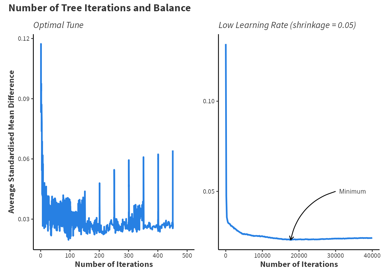

Figure 3.1: Relatoinship between standardised mean difference, number of interations, and learning rate in a GBM model. Please note the difference in horozontal scale between the two learning rates. The model is fit using weightit from the WeightIt package.

For the optimal machine fit, finding that balance worsens as the number of trees increases is just as informative as knowing the correct number of trees. Provided sufficient computational performance, a wide grid search is beneficial in the long run to ensure that each model specification reaches the best balance possible.

3.2.2 Step 7 and 8: Assessing Balance

The Importance of Discussing Balance

Assessing balance is crucial because it ensures that the treated and control groups are comparable on observed covariates. This comparability is essential for reducing confounding and making valid causal inferences. Without proper balance, differences in outcomes between the groups could be due to pre-existing differences rather than the treatment itself. Balance assessment helps to verify that the propensity score model has effectively adjusted for covariates, creating a pseudo-randomised scenario. This step is vital for the reliability and validity of the study’s conclusions. King and Nielsen (2019) notes that many papers that implement propensity score methods do not assess or report a balance in their studies, which can undermine the credibility of the research process and make it hard for readers to understand why results are robust.

A good resource of information for assessing balance is documentation from the cobalt package, which can be viewed by running vignette(“cobalt”, package = “cobalt”) in R.

As stated, cobalt provides very good integration with other related packages such as WeightIt for IPW and MatchIt for propensity score matching. Balance tables are created using bal.tab().

1library(cobalt)
2nsw_logit_btab <- bal.tab(nsw_logit_weight,
                          data = nsw_data,
3                          stats = c("mean.diffs","variance.ratios"),
                          binary = "std", continuous = "std",
4                          thresholds = c(mean.diffs = 0.1))

5nsw_logit_btab <- nsw_logit_btab$Balance[-1,-c(2,3)]

1

Loads the cobalt package. This assumes the package is already installed with install.packages("cobalt")

2

Uses the bal.tab() fucntion to create balance statistics for the previously created nsw_logit_weight model.

3

Specifies the calculation of standardised mean differences and variance ratios for each covariate. The mean differences will be standardised for binary and continuous variables.

4

Sets a threshold of balance to be \(0.1\) to determine if a covariate is balanced.

5

Extracts the balance table of the nsw_logit_btab object and removes excessive columns. This is only completed for ease of visualisation and is not typically required.

Additionally, bal.tab() will create balance tables for the GBM method’s IPWs and the raw data. For presentation, dplyr combines each of the individual balance tables for presentation using kable and kableExtra.

# Create balance tables
nsw_boosted_btab <- bal.tab(nsw_boosted_weight, 
                            data = nsw_data,
                            stats = c("mean.diffs","variance.ratios"),
                            binary = "std", continuous = "std",
                            thresholds = c(mean.diffs = 0.1))

nsw_raw_btab <- bal.tab(nsw_formula, 
                        data = nsw_data, 
                        stats = c("mean.diffs","variance.ratios"),
                        binary = "std", continuous = "std",
                        thresholds = c(mean.diffs = 0.1),
                        s.d.denom = "treated")

nsw_boosted_btab <- nsw_boosted_btab$Balance[-1, -c(2, 3)]
nsw_raw_btab <- nsw_raw_btab$Balance[-c(5, 6)]

# Create Table 3.1
library(tidyverse)
library(kableExtra)

collabels <- c("Type", "SMD", "Balanced", "Variance Ratio","Method")

rowlabels <- c("Age", "Education", "Income 1975","Black", 
               "Hispanic", "Degree", "Married")

nsw_raw_btab$method <- "Raw Data"
nsw_logit_btab$method <- "IPTW: Logistic Regression"
nsw_boosted_btab$method <- "IPTW: Boosting"

combined_btab <- bind_rows(setNames(nsw_raw_btab,collabels),
                           setNames(nsw_logit_btab,collabels),
                           setNames(nsw_boosted_btab,collabels))

combined_btab$Variable <- rep(rowlabels,3)

combined_btab <- combined_btab[c(6,1,2,3,4,5)]

rownames(combined_btab) <- NULL

combined_btab$Balanced <- ifelse(
          combined_btab$Balanced == "Not Balanced, >0.1", "No", "Yes")

kbl(combined_btab[-6], digits = 4, booktabs = TRUE, align = "c", 
      font_size = 10) %>%
  kable_styling(full_width = T) %>%
  column_spec(2:5, bold = F, width = "3cm") %>%
  pack_rows("Raw Data", 1, 7, label_row_css = "text-align: center;") %>%
  pack_rows("Logistic Regression and IPTW", 8, 14, 
             label_row_css = "text-align: center;") %>%
  pack_rows("Boosting Machine and IPTW", 15, 21,
             label_row_css = "text-align: center;")

Table 3.1: Standardised mean difference (a measure of balance) across different covariates in the National Supported Work data. The values are categorised for different propenensity score methods allowing a comparison. Balance tables are computed using bal.tab() from the cobalt package.

Variable	Type	SMD	Balanced	Variance Ratio
Raw Data
Age	Contin.	0.1066	No	1.0278
Education	Contin.	0.1281	No	1.5513
Income 1975	Contin.	0.0824	Yes	1.0763
Black	Binary	0.0449	Yes	NA
Hispanic	Binary	-0.2040	No	NA
Degree	Binary	0.2783	No	NA
Married	Binary	0.0902	Yes	NA
Logistic Regression and IPTW
Age	Contin.	-0.0001	Yes	0.9809
Education	Contin.	0.0012	Yes	1.2725
Income 1975	Contin.	0.0081	Yes	0.7971
Black	Binary	0.0006	Yes	NA
Hispanic	Binary	-0.0031	Yes	NA
Degree	Binary	0.0009	Yes	NA
Married	Binary	0.0045	Yes	NA
Boosting Machine and IPTW
Age	Contin.	-0.0065	Yes	0.9086
Education	Contin.	0.0220	Yes	1.1391
Income 1975	Contin.	-0.0152	Yes	1.0134
Black	Binary	0.0028	Yes	NA
Hispanic	Binary	-0.0547	Yes	NA
Degree	Binary	0.0481	Yes	NA
Married	Binary	0.0085	Yes	NA

Table 3.1 shows that both logistic regression and the GBM have reduced imbalance. The raw data exhibits imbalance across age, years of education, if someone is gispanic, and if someone has a bachelors degree. Imbalanced datasets leads to biased treatment effect estimation so the estimate of the treatment effect in the raw data may be biased. In this example, logistic regression appears to achieve the best covariate balance although GBM achieves slightly better variance ratios.

3.2.3 Step 9: Results

Finally, the treatment effect can be estimated using lm_weightit() from the WeightIt package and avg_comparisons() from the marginaleffects package. Note that the outcome variable is re78 which is real income in 1978 meaning that the income is adjusted for inflation. Previously, the treatment indicator was the outcome variable because the propensity scores are a prediction of the treatment indicator.

1nsw_boosted_lm <- lm_weightit(re78 ~ treat * (age + educ + re75 + black +
                              hisp + degree + marr), data = nsw_data,
2                              weights = nsw_boosted_weight$weights)

3library(marginaleffects)
nsw_boosted_result <- avg_comparisons(nsw_boosted_lm, variables = "treat")

1

Uses lm_weightit() to compute pseudo-outcomes. The formula here specifies an interaction between the treatment and all other variables. Note that * indicates multiplication in R.

2

Specifies the weights from the nsw_boosted_weight object created earlier by the weightit() function. Intuitively, this is performing linear regression using the pseudo-population, where the pseudo-population is created weighting the data by nsw_boosted_weight$weights.

3

Estimates a comparison between the potential outcomes as well as standard errors for inference.

Additionally, this process is followed for the logistic regression propensity scores and the results are combined in to a table for comparison.

# Create Table 3.2
nsw_logit_lm <- lm_weightit(re78~treat*(age + educ + 
                             re75 + black + hisp + 
                             degree + marr), data = nsw_data, 
                             weights = nsw_logit_weight$weights)

nsw_logit_result <- avg_comparisons(nsw_logit_lm, variables = "treat")

nsw_comparisons_tab <- rbind(extract_comparison_results(nsw_logit_result),
                             extract_comparison_results(nsw_boosted_result))
rownames(nsw_comparisons_tab) <- c("Logistic Regression", "GBM")

knitr::kable(nsw_comparisons_tab, digits = 4)

Table 3.2: Comparison of estimates of the average treatment for the National Supported Work data.

	Estimate	SE	P.Value	Lower.CI	Upper.CI
Logistic Regression	1610.786	668.4870	0.0160	300.5756	2920.997
GBM	1609.947	669.4201	0.0162	297.9081	2921.987

Table 3.2 shows that both estimates of the treatment effect are nearly identical at \(\$1610\) with logistic regression inferring a \(\$0.86\) larger treatment effect. Additionally, these results are statistically significant at the \(5\%\) level with nearly identical standard errors.

Friedman, Jerome H. 2001. “Greedy Function Approximation: A Gradient Boosting Machine.” The Annals of Statistics 29 (5): 1189–1232. https://www.jstor.org/stable/2699986.

King, Gary, and Richard Nielsen. 2019. “Why Propensity Scores Should Not Be Used for Matching.” Political Analysis 27 (4): 435–54. https://doi.org/10.1017/pan.2019.11.

McCaffrey, Daniel F., Greg Ridgeway, and Andrew R. Morral. 2004. “Propensity score estimation with boosted regression for evaluating causal effects in observational studies.” Psychological Methods 9 (4): 403–25. https://doi.org/10.1037/1082-989X.9.4.403.

Ridgeway, Greg, Dan Mccaffrey, Andrew Morral, Matthew Cefalu, Lane Burgette, and Beth Ann Griffin. 2024. “Toolkit for Weighting and Analysis of Nonequivalent Groups: A Tutorial for the R TWANG Package.” https://doi.org/10.7249/tl136.1.

Rosenbaum, Paul R., and Donald B. Rubin. 1983. “The central role of the propensity score in observational studies for causal effects.” Biometrika 70 (1): 41–55. https://doi.org/10.1017/CBO9780511810725.016.

---

1. In the context of gradient boosting machines (GBMs) or boosted logistic regression models, an offset refers to an additional term that is included in the model to account for a known effect or baseline value that should be factored into the prediction, but is not estimated by the model itself. In gbm the offset is estimated using conventional logistic regression.