The replication study focuses on a paper titled The Impact of Coffee Certification on Small-Scale Producers’ Livelihoods: A Case Study from the Jimma Zone, Ethiopia published in Agricultural Economics (2012) by Pradyot Ranjan Jena, Bezawit Beyene Chichaibelu, Till Stellmacher, and Ulrike Grote. This paper explores the effects of fair trade coffee certification schemes on the economic wellbeing of small-scale coffee farmers in Ethiopia, particularly examining whether these schemes contribute to poverty reduction and improved livelihoods among smallholders.
The central theme of the paper is the evaluation of certification schemes, such as Fairtrade and organic certification, as tools for enhancing the income stability and economic resilience of small-scale coffee producers. Certification is seen as a potential tool for economic growth and and environmental sustainability and so it is important to understand the impact on small-scale farmers. Table 4.1 summarises the variables used in the propensity score model.
# Create Table 4.1library(dplyr) coffee_variable_summary <-data.frame(Codename =c("`percapinc_day`", "`certified`", "`age_hh`", "`agesq`", "`gender`", "`depratio`", "`edu`", "`experience`", "`logtotal_land`", "`access_credit`", "`badweat`", "`nf_income`"),Description =c("Average income earned per person within a farming household", "If the farming household is certified (1) or otherwise (0)", "Age of the head of the household in years", "Age of the head of the household squared", "Gender of the head of household (male = 1 and female = 0)", "Ratio of adult to childern in household (14 years or less)","Education of the head of household in years","Years of experience in coffee farming","Logarithm of total land size in hectares","Household has access to credit (yes = 1, otherwise = 0)","If the household experienced floods/droughts in 2008–2009","If the household has access to nonfarm income"))rownames(coffee_variable_summary) <-c("Per Capita Income", "Certification (Treatment/ Control)", "Household Age", "Squared Household Age", "Gender", "Dependency Ratio", "Education Level", "Years of Coffee Production", "Log Total Land", "Access to Credit", "Bad Weather", "Non-farm Income Access")knitr::kable(coffee_variable_summary, align="c")
Table 4.1: List of covaraites in Jena et al. (2012). Per capita income is the outcome and certification is the treatment. Other covariates are used in the propensity score model.
Codename
Description
Per Capita Income
percapinc_day
Average income earned per person within a farming household
Certification (Treatment/ Control)
certified
If the farming household is certified (1) or otherwise (0)
Household Age
age_hh
Age of the head of the household in years
Squared Household Age
agesq
Age of the head of the household squared
Gender
gender
Gender of the head of household (male = 1 and female = 0)
Dependency Ratio
depratio
Ratio of adult to childern in household (14 years or less)
Education Level
edu
Education of the head of household in years
Years of Coffee Production
experience
Years of experience in coffee farming
Log Total Land
logtotal_land
Logarithm of total land size in hectares
Access to Credit
access_credit
Household has access to credit (yes = 1, otherwise = 0)
Bad Weather
badweat
If the household experienced floods/droughts in 2008–2009
Non-farm Income Access
nf_income
If the household has access to nonfarm income
Jena et al. (2012) define livelihood as a combination of per capita income, total income, per capita consumption, and yield per hectare. For simplicity, this replication will only use per capita income as a dependent variable. This measure is selected as per capita income is a direct measurement of the income of those potentially impacted by certification. Additionally, the replication uses the same variables as the original paper so any difference in estimates or covariate balance can be attributed to the propensity score model.
Randomisation into certified and uncertified is not possible and it is likely that farmers who seek certification are different than farmers who don’t. Thus, there is selection bias leading to structural differences between groups so a contrast in means between the certified (treated) and uncertified (control) farmers would be biased. Propensity scores are used to create covariate balance and reduce bias of the estimated treatment effect. The paper did not assess the balance of covariates. However, this provides a good opportunity to assess covariate balance in the initial paper and the repeat the analysis using a machine learning propensity model.
4.1 Replication of Original Results
Jena et al. (2012) provides a replication package including Stata code that uses Stata’s psmatch2 package to perform nearest neighbour matching with replacement and common support trimming. Common support trimming means that any observations outside the commonly overlapping are are discarded. The results of the paper are be fully replicated using the MatchIt package inside R.
Table 4.2: Replication of results in Jena et al. (2012). Note a slight difference in standard error which should be \(1.1\) as the MatchItSE package uses a trivially different method than psmatch2 in Stata (see Abadie and Imbens 2006). Matching is performed by matchit() from the MatchIt package.
Estimate
SE
P.Value
Lower.CI
Upper.CI
Replicated Result
-0.1538
0.9898
0.835
-1.6009
1.2934
Table 4.2 shows the replicated result obtained by Jena et al. (2012). The intriguing finding of the paper is that the average treatment effect on the treated (ATT) is negative. That is, of the farmers that become certified, their per capita income is expected to decrease by \(\$0.15\) per day. Intuition and proponents of certification schemes suggest that certification leads to an increase of income. If certification negatively impacts income, it would call into question a significant effort to engage in certification and fair trade practices.
Jena et al. (2012) does not perform any discussion or consideration of balance in their paper and so it is unclear if propensity score matching results in covariate balance. The cobalt package creates balance tables using bal.tab() and a visualisation using love.plot().
Table 4.3: The standardised mean difference (SMD) for each covariate in Jena et al. (2012) using a logistic regression propensity model and propensity score matching. Across each of the covariates, a balance threshold is set at \(0.1\) to indicate if a covariate is balanced. Binary and continuous variables are both standardised over the treatment group. SMDs are computed using bal.tab() from the cobalt package.
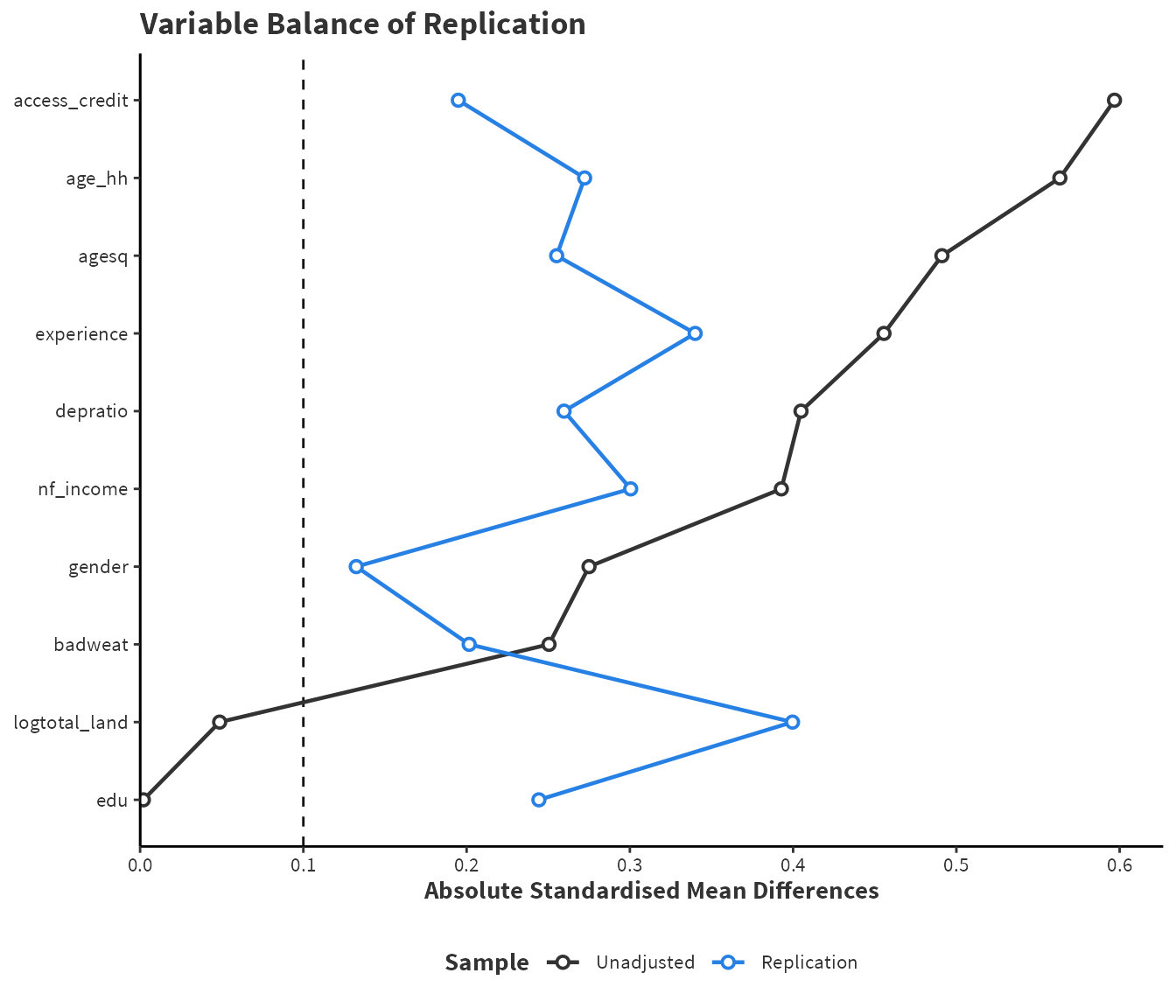
Figure 4.1: A visual representation of Table 4.3 called a love plot. Additionally, the unadjusted (raw data) SMDs are displayed for comparison. Variables are ordered by the SMD in the unadjusted data. Plot is created using love.plot() from the cobalt package.
Table 4.3 and Figure 4.1 show that propensity score matching has obtained very poor balance. Based on the \(0.10\) rule discussed in Section 2.1.1, not a single variable is balanced and so the estimate of the treatment effect is likely to be biased by structural differences between control and certified.
Four key variables: age, gender, education, and access to credit all exhibit poor balance. These variables are strong confounders in theory and so emphasising balance in these variables is critical to making a robust causal inference. Perhaps there is gender or age discrimination in the certification process. Perhaps, those with lesser education may struggle to obtain certification. Perhaps those who have less access to credit are unable to afford to become certified. Moving forward, these variables must exhibit better covariate balance to make a robust conclusion.
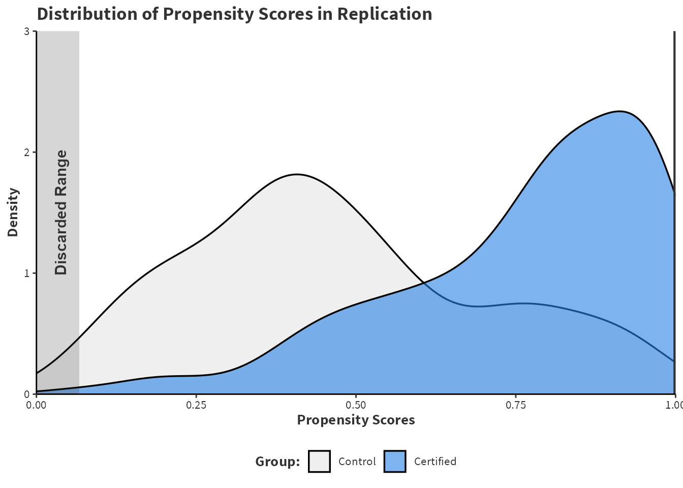
Figure 4.2 shows the effect of common support trimming. Table 4.4 shows 34 total observations are dropped of which 33 are treated and 1 are control. By dropping these observations, PSM avoids making poor matches which should lead to better covariate balance. When observations are discarded, the estimand is no longer the ATT. Instead, it is refereed to as the average treatment effect on the matched or ATM. There is a significant reduction in the effective sample size in the control group from \(82\) to \(21\) individuals.
# Create Figure 4.2discarded_scores <- coffee_rep_pmodel$distance[coffee_rep_pmodel$discarded]discard_min <-min(discarded_scores, na.rm =TRUE)discard_max <-max(discarded_scores, na.rm =TRUE)ggplot(coffee_data, aes(x = coffee_rep_pmodel$distance, fill =factor(certified))) +geom_density(alpha =0.6, linewidth =0.6) +scale_fill_manual(values =c("#e5e5e5", "#2780e3"), labels =c("Control", "Certified")) +labs(title ="Distribution of Propensity Scores in Replication", x ="Propensity Scores", y ="Density", fill ="Group:") +scale_x_continuous(expand =expansion(0), limits =c(0, 1)) +scale_y_continuous(expand =expansion(0), limits =c(0, 3)) +geom_vline(xintercept = discard_max, color ="#333333", linewidth =0.8) +annotate("rect", xmin =0, xmax = discard_min, ymin =-Inf, ymax =Inf, fill ="#333333", alpha =0.2) +annotate("rect", xmin = discard_max, xmax =1, ymin =-Inf, ymax =Inf, fill ="#333333", alpha =0.2) +annotate("text", x =0.02, y =1.5, label ="Discarded Range", angle =90, vjust =1.5, size =4,fontface ="bold", color ="#333333") + custom_ggplot_theme
Figure 4.2: Density estimates of the propensity scores from Jena et al. (2012) using logistic regression. Propensity score matching discards some observations as displayed by the discarded range on the left. A single observation is discarded on the right.
Table 4.4: The effective sample size resulting from the use of propensity score matching in Jena et al. (2012). The effective sample size (ESS) is displayed in the unweighted (raw) and matched data as well as the number of disarded observations. Computed using bal.tab() from the cobalt package.
Control
Certified
All (ESS)
82
164
All (Unweighted)
82
164
Matched (ESS)
21
131
Matched (Unweighted)
42
131
Unmatched
39
0
Discarded
1
33
Overall, the propensity score matching in Jena et al. (2012) is poor and results in unbalanced covariates and a loss of estimand.
4.2 Further Modelling
To improve the poor balance achieved by the Jena et al. (2012), there are two strategies to obtain better balance. First, the propensity scores can be re-estimated using machine learning to obtain better calibrated propensity scores. Second, inverse propensity weighting (IPW) can be used instead of propensity score matching (PSM). IPW should ensure that the sample size remains the same as no observations are lost through a matching process. IPW should retain all observations and preserve the estimand as the ATT. Additionally, IPW is generally more efficient as a pseudo-population is based on precise weights compared to matched observations based on approximate similarity.
The machine learning propensity scores will be estimated using the WeightIt package in the same process as Chapter 3. The model will be used using criterion = "smd.mean" for simplicity.
Code: Perform IPW with a GBM
# Perform IPW with a GBMlibrary(WeightIt)library(cobalt)set.seed(88)coffee_boosted_weight <-weightit(coffee_formula, data = coffee_data, method ="gbm", distribution ="bernoulli",use.offset = T,shrinkage =seq(0.15, 0.4, length.out =5),bag.fraction =0.67, interaction.depth =3:6,n.trees =500,criterion ="smd.mean", estimand ="ATT")coffee_boosted_btab <-bal.tab(coffee_boosted_weight, data = coffee_data, stats =c("mean.diffs", "variance.ratios"),binary ="std", continuous ="std",thresholds =c(mean.diffs =0.1),s.d.denom ="treated")coffee_boosted_btab <- coffee_boosted_btab$Balance[-1, -c(2,3)]
Note 4.1: Discussion of Tuning
Initially, a tuning grid considering shrinkage values of \(0.001,0.005, 0.01, 0.05, 0.1, 0.2, \text{ and }0.3\) were considered using \(10000\) trees with a depth between \(1\) and \(5\). The best tuning performance was found with shrinkage of \(0.2\) and \(13\) trees which were three splits \(2\) deep.
As such my later tuning grids considered higher learning rates and a smaller number of trees. The third and final iteration of the tuning grid searches between \(0.15, 0.2125, 0.275, 0.3375, \text{ and }0.4\), between \(3\) and \(6\) splits deep, uses an offset, and randomly selects \(67\%\) of the data at each tree.
Code: Perform IPW with Logistic Regression
# Perform IPW with Logistic Regressioncoffee_logit_weight <-weightit(coffee_formula, data = coffee_data, method="glm", estimand ="ATT")coffee_logit_btab <-bal.tab(coffee_logit_weight, data = coffee_data,formula = coffee_formula,stats =c("mean.diffs", "variance.ratios"),binary ="std", continuous ="std",thresholds =c(mean.diffs =0.1),s.d.denom ="treated")coffee_logit_btab <- coffee_logit_btab$Balance[-1, -c(2,3)]
Of course there is no guarantee that the GBM model will perform the best and so a logistic model is also fitted. An interesting comparison is between the SMDs in the matched data and in the weighted sample. Any differences between the two samples relates to the difference between PSM and IPW as the propensity scores are identical.
4.3 Comparison of Methods
As before, cobalt creates a balance table and love plot.
Table 4.5: Comparison of standardised mean difference (SMD) using different propensity score models. Across each of the covariates, a balance threshold is set at \(0.1\) to indicate if a covariate is balanced. Binary and continuous variables are both standardised over the treatment group. SMDs are computed using bal.tab() from the cobalt package.
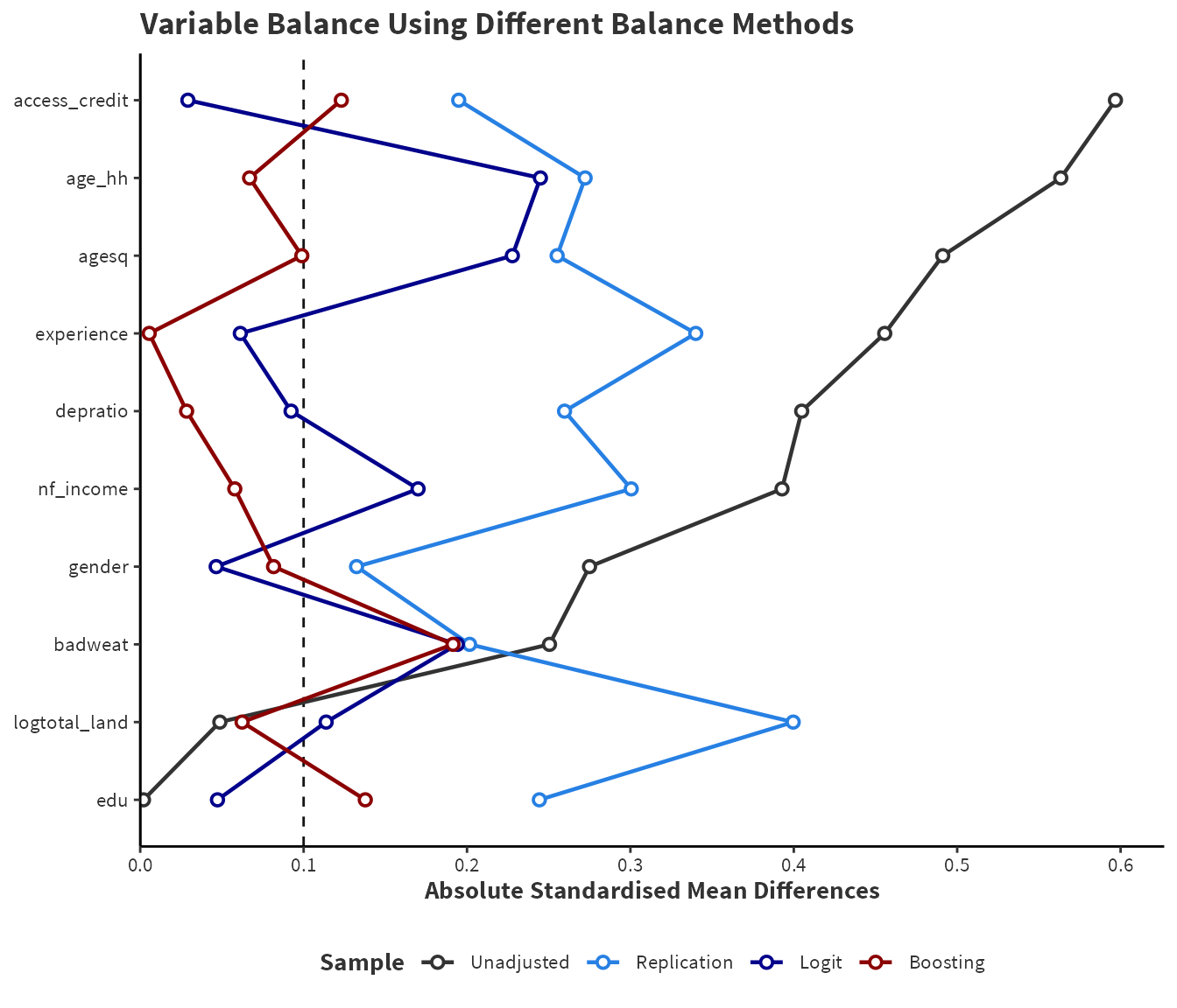
Figure 4.3: Visual representation of Table 4.5 called a love plot and displays the standardised mean difference (SMD) of covariates in Jena et al. (2012). Additionally, the unadjusted SMDs are displayed for comparison. Variables are ordered by the SMD in the unadjusted data.
There are three notable findings:
PSM has performed very poorly relative to IPW even when matching dropps a significant number of observations.
A GBM model has resulted in better covariate balance than logistic regression for most covariates. Using a \(0.1\) guidline for determining balance, logistic regression leaves \(5\) variables unbalanced and the GBM leaves \(3\) variables unbalanced. Additionally, the degree of unbalance is larger for logistic regression.
Logistic regression has a satisfactory average SMD of \(0.077\). Boosting has an average SMD of \(0.0498\) which is excellent and narrowly meets a rigorous threshold of \(0.05\).
The covariate with the highest SMD is household age (\(0.245\)) in logistic regression and bad weather (\(0.191\)) in the GBM.
4.4 Results
Now that satisfactory covariate balance is achieved, the treatment effect can be estimated under logistic regression, the GBM, and then compared to the result in the paper. Note that the estimand in the paper is intended to be the average treatment effect (ATT) but dropped observations mean the actual treatment effect is the average treatment effect on matched (ATM) individuals. In theory, better covariate balance should lead to a better estimate of the ATT so a comparison of the estimates is interesting. As in Section 3.2.3, the results will be completed using G-computation with the lm_weightit() and avg_comparisons() functions.
Table 4.6: Estimates of the average treatment effect on the treated of certification on per capita income across different propensity score models and methods. Created using WeightIt, MatchIt, and Cobalt packages.
Estimate
SE
P.Value
Lower.CI
Upper.CI
Rep. Result (Logistic with PSM)
-0.1538
0.9898
0.8350
-1.6009
1.2934
Logistic Regression and IPW
-1.5824
0.6072
0.0092
-2.7724
-0.3924
Generalized Boosting Machine and IPW
-1.0187
0.5196
0.0499
-2.0372
-0.0003
Table 4.6 shows the estimates of the treatment effect across different methods. Recall that Jena et al. (2012) estimate a an effect of \(-0.15\) implying that daily income reduces by \(\$0.15\) if a farmer becomes certified. This result is not statistically significant.
The IPW estimate is \(-1.58\) implying that certification leads to a \(\$1.58\) decrease in daily income. This coefficient is much larger than than the original paper by a magnitude of \(10\). Additionally, this estimate is statistically significant at the \(1\%\) level. The GBM estimate is \(-1.02\) which predicts a decrease in daily income by \(\$1.02\) when a farmer becomes certified. This finding is statistically significant at the \(5\%\) level.
The most interesting result is that the estimates become even more negative. One may expect that the result from a better balanced sample would become positive to align with theoretical motivations for certification policies. Jena et al. (2012) presented two explanations for why certification shows no positive impact. First, the authors note that the prices offered by certified cooperatives are not significantly different from those provided by non-certified cooperatives. Second, a substantial portion of coffee—about \(75\%\) is sold to private traders, who often pay higher prices to non-certified farmers. Additionally, from qualitative interviews with farmers, the authors note that policies and arrangements within different cooperatives exhibit heterogeneity so the impact of certification may relate more to the structure of the cooperatives not merely being certified.
The reason for a large difference is twofold. First, better covariate balance by using a GBM and IPW and should result in a more robust estimate. Of course better covariate balance alone does not guarantee robust results but it is a step in the right direction. Second, weighting on the inverse of the propensity scores instead of matching may significantly effect the estimate of the treatment effect especially when matching results in dropped observations.
An additional answer is the impact of reverse causality. A general problem is causal inference is that the direction of causality is not always known. While it is most intuitive that coffee certification would impact income, it is also possible that per capita income might determine their certification. Suppose that proponents of fair trade and certification are correct that certification will increase income and benefit livelihood. If farmers are aware of this, then perhaps the lowest income farmers are most likely to attempt to become certified to increase their income. Additionally, income likely has a reverse causal relationship with many of the explanatory variables. For example, a higher income may lead to better access to credit and the accumulation of land.
In summary, the analysis demonstrates that using more advanced methods like GBM and IPW not only improves covariate balance but also leads to significantly larger and more negative estimates of the treatment effect compared to the original study. This suggests that previous estimates may have underestimated the negative impact of certification on per capita income. The findings highlight the importance of methodological rigor in estimating causal effects and raise critical questions about the broader implications of certification policies, particularly when considering potential reverse causality and the varying structures of cooperatives. This analysis underscores the need for careful interpretation of treatment effects, especially in policy-relevant research.
Abadie, Alberto, and Guido W. Imbens. 2006. “Large sample properties of matching estimators for average treatment effects.”Econometrica 74 (1): 235–67. https://doi.org/10.1111/j.1468-0262.2006.00655.x.
Jena, Pradyot Ranjan, Bezawit Beyene Chichaibelu, Till Stellmacher, and Ulrike Grote. 2012. “The impact of coffee certification on small-scale producers’ livelihoods: A case study from the Jimma Zone, Ethiopia.”Agricultural Economics (United Kingdom) 43 (4): 429–40. https://doi.org/10.1111/j.1574-0862.2012.00594.x.
Source Code
# Replication Case Study {#sec-replication}```{r}#| include: falseload(file ="globals.RData")```The replication study focuses on a paper titled *The Impact of Coffee Certification on Small-Scale Producers' Livelihoods: A Case Study from the Jimma Zone, Ethiopia* published in Agricultural Economics (2012) by Pradyot Ranjan Jena, Bezawit Beyene Chichaibelu, Till Stellmacher, and Ulrike Grote. This paper explores the effects of fair trade coffee certification schemes on the economic wellbeing of small-scale coffee farmers in Ethiopia, particularly examining whether these schemes contribute to poverty reduction and improved livelihoods among smallholders.The central theme of the paper is the evaluation of certification schemes, such as Fairtrade and organic certification, as tools for enhancing the income stability and economic resilience of small-scale coffee producers. Certification is seen as a potential tool for economic growth and and environmental sustainability and so it is important to understand the impact on small-scale farmers. @tbl-coffee-var-summary summarises the variables used in the propensity score model. ```{r }#| label: tbl-coffee-var-summary#| code-fold: true#| echo: !expr "knitr::is_html_output()"#| code-summary: "Code: Create [Table 4.1](#tbl-coffee-var-summary)"#| tbl-cap: "List of covaraites in @Jena2012. Per capita income is the outcome and certification is the treatment. Other covariates are used in the propensity score model."# Create Table 4.1library(dplyr) coffee_variable_summary <- data.frame( Codename = c("`percapinc_day`", "`certified`", "`age_hh`", "`agesq`", "`gender`", "`depratio`", "`edu`", "`experience`", "`logtotal_land`", "`access_credit`", "`badweat`", "`nf_income`"), Description = c("Average income earned per person within a farming household", "If the farming household is certified (1) or otherwise (0)", "Age of the head of the household in years", "Age of the head of the household squared", "Gender of the head of household (male = 1 and female = 0)", "Ratio of adult to childern in household (14 years or less)", "Education of the head of household in years", "Years of experience in coffee farming", "Logarithm of total land size in hectares", "Household has access to credit (yes = 1, otherwise = 0)", "If the household experienced floods/droughts in 2008–2009", "If the household has access to nonfarm income"))rownames(coffee_variable_summary) <- c("Per Capita Income", "Certification (Treatment/ Control)", "Household Age", "Squared Household Age", "Gender", "Dependency Ratio", "Education Level", "Years of Coffee Production", "Log Total Land", "Access to Credit", "Bad Weather", "Non-farm Income Access")knitr::kable(coffee_variable_summary, align="c")```@Jena2012 define livelihood as a combination of per capita income, total income, per capita consumption, and yield per hectare. For simplicity, this replication will only use per capita income as a dependent variable. This measure is selected as per capita income is a direct measurement of the income of those potentially impacted by certification. Additionally, the replication uses the same variables as the original paper so any difference in estimates or covariate balance can be attributed to the propensity score model. Randomisation into certified and uncertified is not possible and it is likely that farmers who seek certification are different than farmers who don't. Thus, there is selection bias leading to structural differences between groups so a contrast in means between the certified (treated) and uncertified (control) farmers would be biased. Propensity scores are used to create covariate balance and reduce bias of the estimated treatment effect. The paper did not assess the balance of covariates. However, this provides a good opportunity to assess covariate balance in the initial paper and the repeat the analysis using a machine learning propensity model. ## Replication of Original Results@Jena2012 provides a replication package including Stata code that uses Stata's psmatch2 package to perform nearest neighbour matching with replacement and common support trimming. Common support trimming means that any observations outside the commonly overlapping are are discarded. The results of the paper are be fully replicated using the `MatchIt` package inside R.```{r }#| label: tbl-replicated-result#| code-fold: true#| echo: !expr "knitr::is_html_output()"#| code-summary: "Code: Create [Table 4.2](#tbl-replicated-result)"#| tbl-cap: "Replication of results in @Jena2012. Note a slight difference in standard error which should be $1.1$ as the `MatchItSE` package uses a trivially different method than psmatch2 in Stata [see @Abadie2006]. Matching is performed by `matchit()` from the `MatchIt` package."# Create Table 4.2library(MatchIt)library(MatchItSE)library(marginaleffects)coffee_formula <- as.formula(certified ~ age_hh + agesq + nf_income + depratio + logtotal_land + badweat + edu + gender + experience + access_credit)coffee_rep_pmodel <- matchit(coffee_formula, data = coffee_data, distance = "glm", method = "nearest", replace = TRUE, estimand = "ATT", discard = "both") coffee_logit_md <- match.data(coffee_rep_pmodel)coffee_rep_fit<- lm(percapinc_day ~ certified, data = coffee_logit_md, weights = weights)replicated_result <- avg_comparisons(coffee_rep_fit, variables = "certified", vcov = NULL, newdata = subset(coffee_logit_md, certified == 1), wts = "weights")ai_se <- abadie_imbens_se(obj = coffee_rep_pmodel, Y = coffee_data$percapinc_day)replicated_result_tbl <- extract_comparison_results(replicated_result)replicated_result_tbl$SE <- ai_serownames(replicated_result_tbl) <- "Replicated Result"knitr::kable(replicated_result_tbl, digits = 4)```@tbl-replicated-result shows the replicated result obtained by @Jena2012. The intriguing finding of the paper is that the average treatment effect on the treated (ATT) is negative. That is, of the farmers that become certified, their per capita income is expected to decrease by $\$0.15$ per day. Intuition and proponents of certification schemes suggest that certification leads to an increase of income. If certification negatively impacts income, it would call into question a significant effort to engage in certification and fair trade practices.@Jena2012 does not perform any discussion or consideration of balance in their paper and so it is unclear if propensity score matching results in covariate balance. The `cobalt` package creates balance tables using `bal.tab()` and a visualisation using `love.plot()`. ```{r}#| label: tbl-coffee-balance#| code-fold: true#| echo: !expr "knitr::is_html_output()"#| code-summary: "Code: Create [Table 4.3](#tbl-coffee-balance)"#| tbl-cap: "The standardised mean difference (SMD) for each covariate in @Jena2012 using a logistic regression propensity model and propensity score matching. Across each of the covariates, a balance threshold is set at $0.1$ to indicate if a covariate is balanced. Binary and continuous variables are both standardised over the treatment group. SMDs are computed using `bal.tab()` from the `cobalt` package."# Create Table 4.3library(cobalt)coffee_rep_btab <-bal.tab(coffee_rep_pmodel, data = coffee_data, stats =c("mean.diffs","variance.ratios"),binary ="std", continuous ="std",thresholds =c(mean.diffs =0.1),s.d.denom ="treated")coffee_rep_btab_ss <- coffee_rep_btab$Observationscoffee_rep_btab <- coffee_rep_btab$Balance[-1,-c(2,3)]rowlabels <-c("Household Age", "Squared Household Age", "Non-farm Income Access", "Log Total Land", "Dependency Ratio", "Bad Weather","Education Level", "Gender", "Years of Coffee Production", "Access to Credit")colnames <-c("Variable","Type", "SMD", "Balance Threshold", "Variance Ratio")rownames(coffee_rep_btab) <- rowlabelscoffee_rep_btab[,3] <-ifelse( coffee_rep_btab[,3] >="Not Balanced, >0.1", "No", "Yes")knitr::kable(coffee_rep_btab, digits =4, align ="c")``````{r}#| include: false#| warning: false#| label: getndroppednobs_coffee_dropped <-sum(coffee_rep_pmodel$discarded, na.rm=TRUE)coffee_data$discarded <- coffee_rep_pmodel$discardednobs_coffee_Tdropped <-nrow(subset(coffee_data,discarded==TRUE&certified==1))nobs_coffee_Cdropped <-nrow(subset(coffee_data,discarded==TRUE&certified==0))``````{r}#| dev: "ragg_png"#| label: fig-coffee-replication-lplot#| code-fold: true#| fig-height: 6#| echo: !expr "knitr::is_html_output()"#| code-summary: "Code: Create [Figure 4.1](#fig-coffee-replication-lplot)"#| fig-cap: "A visual representation of @tbl-coffee-balance called a love plot. Additionally, the unadjusted (raw data) SMDs are displayed for comparison. Variables are ordered by the SMD in the unadjusted data. Plot is created using `love.plot()` from the `cobalt` package."# Create Figure 4.1library(ggplot2)love.plot(coffee_formula, data = coffee_data, weights =list(Replication = coffee_rep_pmodel),sample.names =c("Unadjusted", "Replication"),var.order ="unadjusted", binary ="std",abs =TRUE, colors =c("#333333", "#2780e3"), shapes =c("circle filled", "circle filled"),line =TRUE, thresholds =0.1, s.d.denom ="treated") +labs(title ="Variable Balance of Replication",x ="Absolute Standardised Mean Differences", fill ="Method") +scale_x_continuous(breaks =seq(0,0.6,length.out=7),expand =expansion(c(0, 0.05))) + custom_ggplot_theme ```@tbl-coffee-balance and @fig-coffee-replication-lplot show that propensity score matching has obtained very poor balance. Based on the $0.10$ rule discussed in @sec-assessing-balance, not a single variable is balanced and so the estimate of the treatment effect is likely to be biased by structural differences between control and certified.Four key variables: *age*, *gender*, *education*, and *access to credit* all exhibit poor balance. These variables are strong confounders in theory and so emphasising balance in these variables is critical to making a robust causal inference. Perhaps there is gender or age discrimination in the certification process. Perhaps, those with lesser education may struggle to obtain certification. Perhaps those who have less access to credit are unable to afford to become certified. Moving forward, these variables must exhibit better covariate balance to make a robust conclusion.@fig-replication-pscore shows the effect of common support trimming. @tbl-coffee-replication-ss shows `{r} nobs_coffee_dropped` total observations are dropped of which `{r} nobs_coffee_Tdropped` are treated and `{r} nobs_coffee_Cdropped` are control. By dropping these observations, PSM avoids making poor matches which should lead to better covariate balance. When observations are discarded, the estimand is no longer the ATT. Instead, it is refereed to as the average treatment effect on the matched or ATM. There is a significant reduction in the effective sample size in the control group from $82$ to $21$ individuals. ```{r}#| dev: "ragg_png"#| label: fig-replication-pscore#| code-fold: true#| fig-height: 5#| echo: !expr "knitr::is_html_output()"#| code-summary: "Code: Create [Figure 4.2](#fig-replication-pscore)"#| fig-cap: "Density estimates of the propensity scores from @Jena2012 using logistic regression. Propensity score matching discards some observations as displayed by the discarded range on the left. A single observation is discarded on the right."# Create Figure 4.2discarded_scores <- coffee_rep_pmodel$distance[coffee_rep_pmodel$discarded]discard_min <-min(discarded_scores, na.rm =TRUE)discard_max <-max(discarded_scores, na.rm =TRUE)ggplot(coffee_data, aes(x = coffee_rep_pmodel$distance, fill =factor(certified))) +geom_density(alpha =0.6, linewidth =0.6) +scale_fill_manual(values =c("#e5e5e5", "#2780e3"), labels =c("Control", "Certified")) +labs(title ="Distribution of Propensity Scores in Replication", x ="Propensity Scores", y ="Density", fill ="Group:") +scale_x_continuous(expand =expansion(0), limits =c(0, 1)) +scale_y_continuous(expand =expansion(0), limits =c(0, 3)) +geom_vline(xintercept = discard_max, color ="#333333", linewidth =0.8) +annotate("rect", xmin =0, xmax = discard_min, ymin =-Inf, ymax =Inf, fill ="#333333", alpha =0.2) +annotate("rect", xmin = discard_max, xmax =1, ymin =-Inf, ymax =Inf, fill ="#333333", alpha =0.2) +annotate("text", x =0.02, y =1.5, label ="Discarded Range", angle =90, vjust =1.5, size =4,fontface ="bold", color ="#333333") + custom_ggplot_theme``````{r}#| label: tbl-coffee-replication-ss#| code-fold: true#| echo: !expr "knitr::is_html_output()"#| code-summary: "Code: Create [Table 4.4](#tbl-coffee-replication-ss)"#| tbl-cap: "The effective sample size resulting from the use of propensity score matching in @Jena2012. The effective sample size (ESS) is displayed in the unweighted (raw) and matched data as well as the number of disarded observations. Computed using `bal.tab()` from the `cobalt` package."# Create Table 4.4colnames(coffee_rep_btab_ss) <-c("Control", "Certified")knitr::kable(coffee_rep_btab_ss, digits=0, align ="c")```Overall, the propensity score matching in @Jena2012 is poor and results in unbalanced covariates and a loss of estimand.## Further Modelling To improve the poor balance achieved by the @Jena2012, there are two strategies to obtain better balance. First, the propensity scores can be re-estimated using machine learning to obtain better calibrated propensity scores. Second, inverse propensity weighting (IPW) can be used instead of propensity score matching (PSM). IPW should ensure that the sample size remains the same as no observations are lost through a matching process. IPW should retain all observations and preserve the estimand as the ATT. Additionally, IPW is generally more efficient as a pseudo-population is based on precise weights compared to matched observations based on approximate similarity.The machine learning propensity scores will be estimated using the `WeightIt` package in the same process as @sec-demo. The model will be used using `criterion = "smd.mean"` for simplicity. ```{r}#| label: coffee-boost-btab#| code-fold: true#| echo: !expr "knitr::is_html_output()"#| code-summary: "Code: Perform IPW with a GBM"# Perform IPW with a GBMlibrary(WeightIt)library(cobalt)set.seed(88)coffee_boosted_weight <-weightit(coffee_formula, data = coffee_data, method ="gbm", distribution ="bernoulli",use.offset = T,shrinkage =seq(0.15, 0.4, length.out =5),bag.fraction =0.67, interaction.depth =3:6,n.trees =500,criterion ="smd.mean", estimand ="ATT")coffee_boosted_btab <-bal.tab(coffee_boosted_weight, data = coffee_data, stats =c("mean.diffs", "variance.ratios"),binary ="std", continuous ="std",thresholds =c(mean.diffs =0.1),s.d.denom ="treated")coffee_boosted_btab <- coffee_boosted_btab$Balance[-1, -c(2,3)]```::: {#nte-tuning .callout-note title="Discussion of Tuning"}Initially, a tuning grid considering shrinkage values of $0.001,0.005, 0.01, 0.05, 0.1, 0.2, \text{ and }0.3$ were considered using $10000$ trees with a depth between $1$ and $5$. The best tuning performance was found with shrinkage of $0.2$ and $13$ trees which were three splits $2$ deep. As such my later tuning grids considered higher learning rates and a smaller number of trees. The third and final iteration of the tuning grid searches between $0.15, 0.2125, 0.275, 0.3375, \text{ and }0.4$, between $3$ and $6$ splits deep, uses an offset, and randomly selects $67\%$ of the data at each tree.:::```{r}#| label: coffee_logit_weight#| code-fold: true#| echo: !expr "knitr::is_html_output()"#| code-summary: "Code: Perform IPW with Logistic Regression"# Perform IPW with Logistic Regressioncoffee_logit_weight <-weightit(coffee_formula, data = coffee_data, method="glm", estimand ="ATT")coffee_logit_btab <-bal.tab(coffee_logit_weight, data = coffee_data,formula = coffee_formula,stats =c("mean.diffs", "variance.ratios"),binary ="std", continuous ="std",thresholds =c(mean.diffs =0.1),s.d.denom ="treated")coffee_logit_btab <- coffee_logit_btab$Balance[-1, -c(2,3)]```Of course there is no guarantee that the GBM model will perform the best and so a logistic model is also fitted. An interesting comparison is between the SMDs in the matched data and in the weighted sample. Any differences between the two samples relates to the difference between PSM and IPW as the propensity scores are identical.## Comparison of Methods As before, `cobalt` creates a balance table and love plot. ```{r}#| code-fold: true#| echo: !expr "knitr::is_html_output()"#| code-summary: "Code: Create [Table 4.5](#tbl-coffee-comparison)."#| label: tbl-coffee-comparison#| tbl-cap: "Comparison of standardised mean difference (SMD) using different propensity score models. Across each of the covariates, a balance threshold is set at $0.1$ to indicate if a covariate is balanced. Binary and continuous variables are both standardised over the treatment group. SMDs are computed using `bal.tab()` from the `cobalt` package."# Create Table 4.5library("data.table")library(cobalt)library(kableExtra)library(tidyverse)coffee_raw_btab <-bal.tab(coffee_formula, data = coffee_data, stats =c("mean.diffs","variance.ratios"),binary ="std", continuous ="std",thresholds =c(mean.diffs =0.1),s.d.denom ="treated")coffee_raw_btab <- coffee_raw_btab$Balance[,-c(5,6)]coffee_combined_btab <-rbindlist(list(coffee_raw_btab, coffee_logit_btab, coffee_boosted_btab), use.names =FALSE)coffee_combined_btab$Variable <-rep(rowlabels, 3)coffee_combined_btab <- coffee_combined_btab[, c(5, 1, 2, 3, 4)]coffee_combined_btab[, 4] <-ifelse( coffee_combined_btab[, 4] >="Not Balanced, >0.1", "No", "Yes")kbl(coffee_combined_btab, digits =4, booktabs =TRUE, align ="c", font_size =10, col.names = colnames) %>%kable_styling(full_width =TRUE) %>%column_spec(2:5, bold =FALSE, width ="2cm") %>%pack_rows("Raw Data", 1, 10, label_row_css ="text-align: center;") %>%pack_rows("Logistic Regression and IPTW", 11, 20, label_row_css ="text-align: center;") %>%pack_rows("Boosting Machine with IPTW", 21, 30, label_row_css ="text-align: center;")``````{r}#| dev: "ragg_png"#| label: fig-coffee-love-all#| code-fold: true#| fig-height: 6#| echo: !expr "knitr::is_html_output()"#| code-summary: "Code: Create [Figure 4.3](#fig-coffee-love-all)"#| fig-cap: "Visual representation of @tbl-coffee-comparison called a love plot and displays the standardised mean difference (SMD) of covariates in @Jena2012. Additionally, the unadjusted SMDs are displayed for comparison. Variables are ordered by the SMD in the unadjusted data."# Create Figure 4.3love.plot(coffee_formula,data = coffee_data, weights =list(Replication = coffee_rep_pmodel,Logit = coffee_logit_weight,Boosting= coffee_boosted_weight),var.order ="unadjusted", binary ="std", continuous ="std",abs =TRUE, colors =c("#333333", "#2780e3", "darkblue","darkred"), shapes =rep("circle filled", 4),line =TRUE, thresholds =0.1, s.d.denom ="treated", use.grid = F) +labs(title ="Variable Balance Using Different Balance Methods",x ="Absolute Standardised Mean Differences",fill ="Method") +scale_x_continuous(breaks =seq(0,0.6,length.out=7),expand =expansion(c(0, 0.05))) + custom_ggplot_theme ```There are three notable findings: 1. PSM has performed very poorly relative to IPW even when matching dropps a significant number of observations. 2. A GBM model has resulted in better covariate balance than logistic regression for most covariates. Using a $0.1$ guidline for determining balance, logistic regression leaves $5$ variables unbalanced and the GBM leaves $3$ variables unbalanced. Additionally, the degree of unbalance is larger for logistic regression. 3. Logistic regression has a satisfactory average SMD of $0.077$. Boosting has an average SMD of $0.0498$ which is excellent and narrowly meets a rigorous threshold of $0.05$. 4. The covariate with the highest SMD is *household age* ($0.245$) in logistic regression and *bad weather* ($0.191$) in the GBM.## ResultsNow that satisfactory covariate balance is achieved, the treatment effect can be estimated under logistic regression, the GBM, and then compared to the result in the paper. Note that the estimand in the paper is intended to be the average treatment effect (ATT) but dropped observations mean the actual treatment effect is the average treatment effect on matched (ATM) individuals. In theory, better covariate balance should lead to a better estimate of the ATT so a comparison of the estimates is interesting. As in @sec-nsw-results, the results will be completed using G-computation with the `lm_weightit()` and `avg_comparisons()` functions.```{r}#| code-fold: true#| echo: !expr "knitr::is_html_output()"#| code-summary: "Code: Create [Table 4.6](#tbl-comparison-coffee-results)"#| label: tbl-comparison-coffee-results#| tbl-cap: "Estimates of the average treatment effect on the treated of certification on per capita income across different propensity score models and methods. Created using `WeightIt`, `MatchIt`, and `Cobalt` packages."# Create Table 4.6coffee_att_formula <-update.formula(as.formula(paste("~", paste(attr(terms(coffee_formula), "term.labels"), collapse =" + "))), percapinc_day ~ certified * .)coffee_logit_fit <-lm_weightit(coffee_att_formula,data = coffee_data, weightit = coffee_logit_weight)coffee_boosted_fit <-lm_weightit(coffee_att_formula,data = coffee_data, weightit = coffee_boosted_weight)coffee_logit_att <-avg_comparisons(coffee_logit_fit, variables ="certified")coffee_boosted_att <-avg_comparisons(coffee_boosted_fit, variables ="certified")coffee_comparisons_tab <-rbind(replicated_result_tbl, extract_comparison_results(coffee_logit_att),extract_comparison_results(coffee_boosted_att))rownames(coffee_comparisons_tab) <-c("Rep. Result (Logistic with PSM)","Logistic Regression and IPW", "Generalized Boosting Machine and IPW")knitr::kable(coffee_comparisons_tab, digits =4)```@tbl-comparison-coffee-results shows the estimates of the treatment effect across different methods. Recall that @Jena2012 estimate a an effect of $-0.15$ implying that daily income reduces by $\$0.15$ if a farmer becomes certified. This result is not statistically significant. The IPW estimate is $-1.58$ implying that certification leads to a $\$1.58$ decrease in daily income. This coefficient is much larger than than the original paper by a magnitude of $10$. Additionally, this estimate is statistically significant at the $1\%$ level. The GBM estimate is $-1.02$ which predicts a decrease in daily income by $\$1.02$ when a farmer becomes certified. This finding is statistically significant at the $5\%$ level. The most interesting result is that the estimates become even more negative. One may expect that the result from a better balanced sample would become positive to align with theoretical motivations for certification policies. @Jena2012 presented two explanations for why certification shows no positive impact. First, the authors note that the prices offered by certified cooperatives are not significantly different from those provided by non-certified cooperatives. Second, a substantial portion of coffee—about $75\%$ is sold to private traders, who often pay higher prices to non-certified farmers. Additionally, from qualitative interviews with farmers, the authors note that policies and arrangements within different cooperatives exhibit heterogeneity so the impact of certification may relate more to the structure of the cooperatives not merely being certified.The reason for a large difference is twofold. First, better covariate balance by using a GBM and IPW and should result in a more robust estimate. Of course better covariate balance alone does not guarantee robust results but it is a step in the right direction. Second, weighting on the inverse of the propensity scores instead of matching may significantly effect the estimate of the treatment effect especially when matching results in dropped observations. An additional answer is the impact of reverse causality. A general problem is causal inference is that the direction of causality is not always known. While it is most intuitive that coffee certification would impact income, it is also possible that per capita income might determine their certification. Suppose that proponents of fair trade and certification are correct that certification will increase income and benefit livelihood. If farmers are aware of this, then perhaps the lowest income farmers are most likely to attempt to become certified to increase their income. Additionally, income likely has a reverse causal relationship with many of the explanatory variables. For example, a higher income may lead to better access to credit and the accumulation of land. In summary, the analysis demonstrates that using more advanced methods like GBM and IPW not only improves covariate balance but also leads to significantly larger and more negative estimates of the treatment effect compared to the original study. This suggests that previous estimates may have underestimated the negative impact of certification on per capita income. The findings highlight the importance of methodological rigor in estimating causal effects and raise critical questions about the broader implications of certification policies, particularly when considering potential reverse causality and the varying structures of cooperatives. This analysis underscores the need for careful interpretation of treatment effects, especially in policy-relevant research.::: {.content-visible when-format="pdf"}## Code Provided for PDF Output```{r get-labels, echo = FALSE}labs = knitr::all_labels()labs = setdiff(labs, c("get-labels"))``````{r all-code, ref.label=labs, eval=FALSE}```:::```{r}#| include: falsesave.image(file ="globals.RData")```